Introduction

For a fixed integer $N \geq 2$, consider the array whose $(x, y)$-entry is the residue of $xy$ modulo $N$, where $1 \leq x, y \leq N-1$. This is the multiplication table modulo $N$, which we abbreviate as MTMN. The starting data is therefore entirely finite and arithmetic: one studies multiplication on the positive integers $1,\ldots,N-1$ and then asks what survives after passing to residues. Each residue class -- that is, each possible remainder $a \in \{0, 1, \ldots, N-1\}$ -- determines a set of lattice points

$$A_{N,a} = \{(x, y) \in \{1, \ldots, N-1\}^2 : xy \equiv a \pmod{N}\}.$$

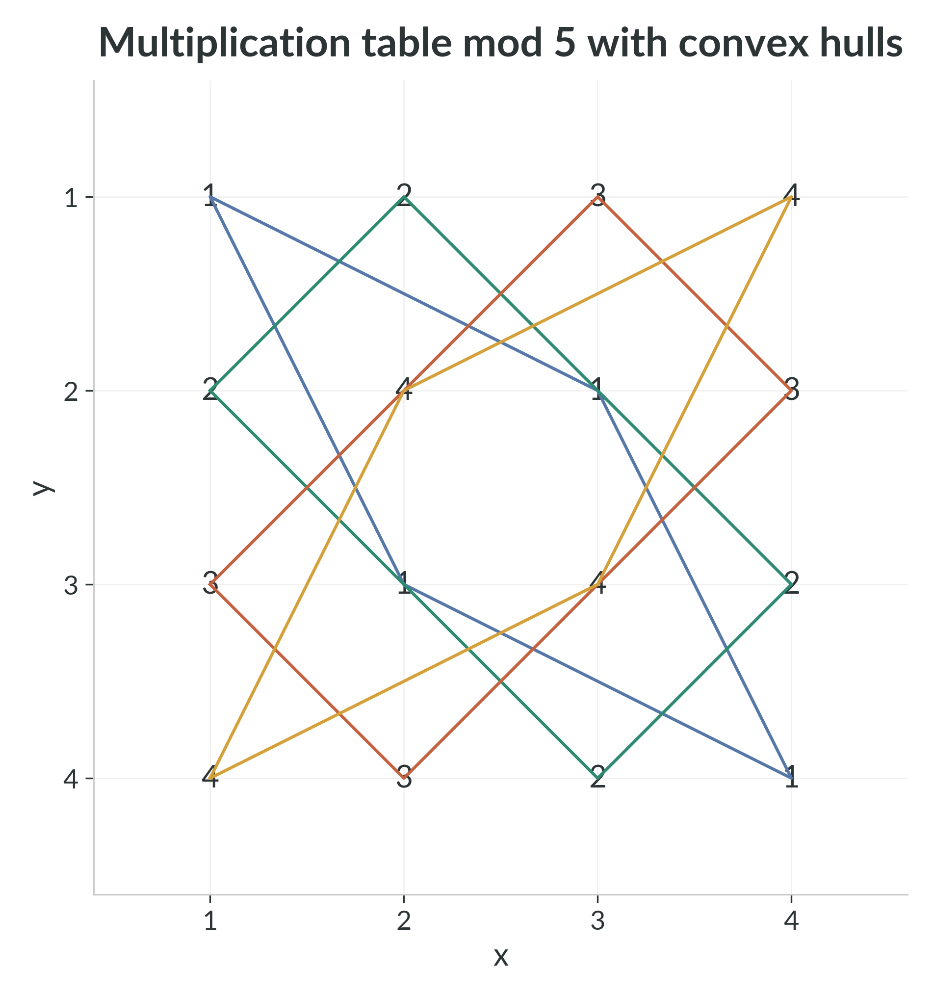
@fig:mtmn-grid-n5 shows a concrete example: the multiplication table modulo $5$, with the convex hull of each residue class overlaid. This is the basic geometric picture that the rest of the book develops.

Multiplication table modulo $5$ with convex hulls of all residue classes. Each colored polygon encloses the lattice points sharing a common residue.

The central geometric quantity of this book is the area of the convex hull of $A_{N,a}$.

Definition (Main area functions). For $N \geq 2$ and $a \in \{0, 1, \ldots, N-1\}$, define $$S(N, a) := \operatorname{Area}(\operatorname{conv}(A_{N,a})).$$ The total area sum is $$S(N) := \sum_{a=0}^{N-1} S(N, a).$$

Each fixed set $A_{N,a}$ is a finite modular hyperbola inside the positive-integer lattice window. Sets of this form have already been studied under that name in the number-theory literature [@shparlinski2012]. The distinctive emphasis of MTMN is different: one studies the whole family of these congruence classes at once, compares their convex hulls residue by residue, and treats the resulting area data as a geometric object in its own right.

There is also a second historical backdrop nearby: the classical Erd\H{o}s multiplication table problem for ordinary integer products. In that setting one asks how many distinct integers appear in an $N \times N$ multiplication table, and later work such as Koukoulopoulos's generalized multiplication-table paper develops the asymptotic distinct-product side of that story [@koukoulopoulos2014]. The guiding contrast is not that MTMN answers the same question in a modular setting, but that it studies a different global invariant. The classical problem concerns distinct ordinary products and shows that this quantity grows more slowly than the naive quadratic scale. MTMN instead studies the summed residue-wise convex-hull area $S(N)$, whose first global theorem already has cubic order of growth. The thematic connection is that both problems ask how much global structure survives inside a multiplication table once multiplication creates many arithmetic coincidences.

That point of view quickly opens into a larger story. A single residue class already has visible Euclidean shape; the whole table can be built border by border from simple modular progressions; and the arithmetic split between coprime and non-coprime indices produces two genuinely different geometric regimes. The next chapters first place this picture beside earlier work on modular hyperbolas, then develop the basic geometry of the residue classes, and then use the zero class to show how divisor geometry and the continuous hyperbola $y=N/x$ meet in one exact area decomposition. After that, the later chapters turn those geometric pictures into exact language: nonzero coprime classes become permutation plots, support functions encode hulls direction by direction, outer rings become exact boundary-layer models, and residue-area packages begin to organize the data algebraically.

Between the discrete set $A_{N,a}$ and its convex hull there is also a natural straight-line intermediate object, treated in Chapter 5 under the name Connecting Residue Points. That same chapter introduces the layer-by-layer construction of the table, the first complete worked examples ($N=5$ and $N=6$), the divisor-controlled zero-class hull, and the hyperbolic correction term $\Delta_N$, so the reader sees concrete geometry before the later exact formulas and asymptotic questions.

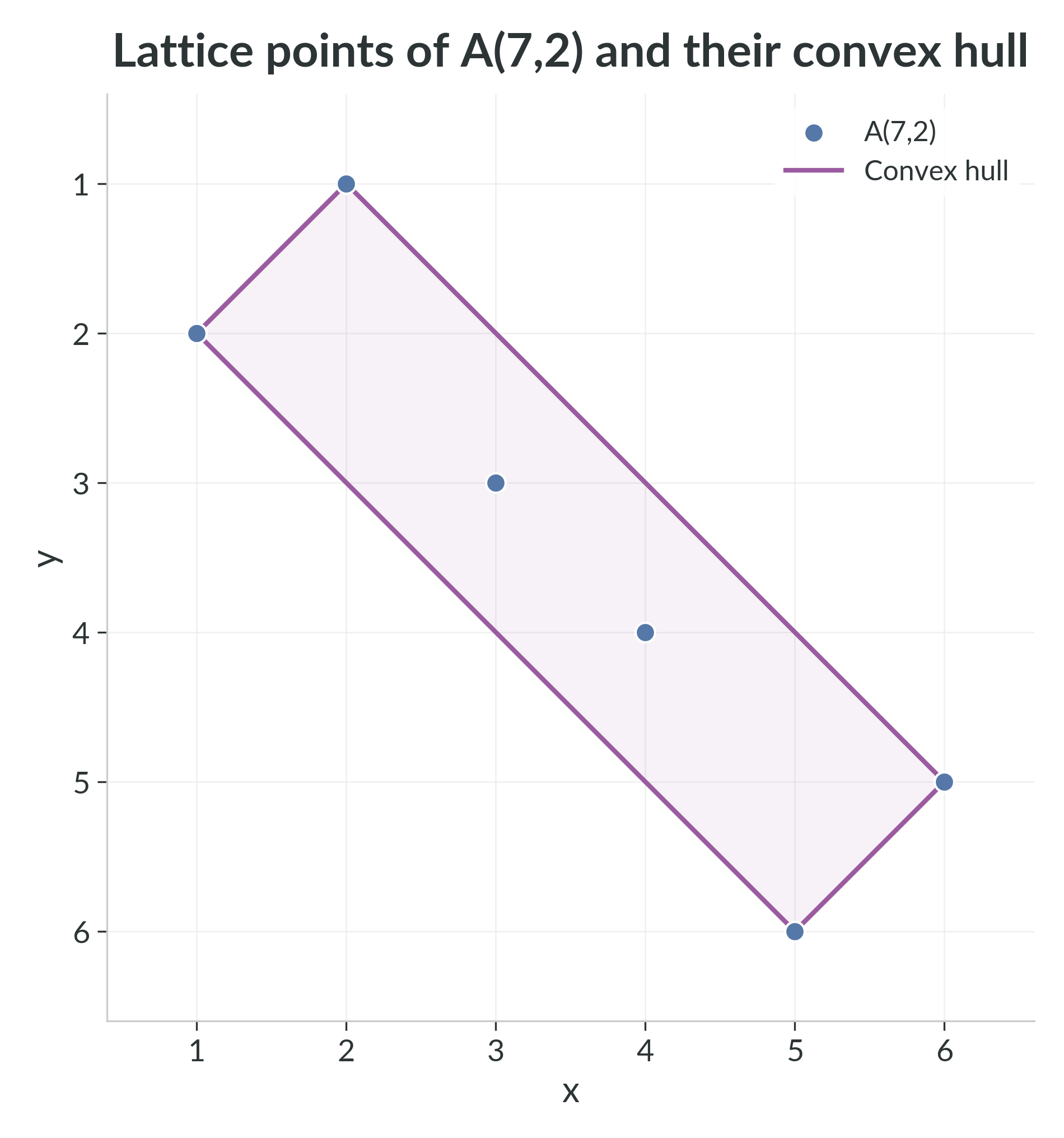
Before turning to the wider program, it helps to look at one residue class by itself. In @fig:lattice-hull-intro the set $A_{7,2}$ appears as a small finite cloud whose convex hull is already a visible polygon. This is the local picture that the whole subject keeps refining: first identify the arithmetic point set, then understand which of those points survive as geometric vertices.

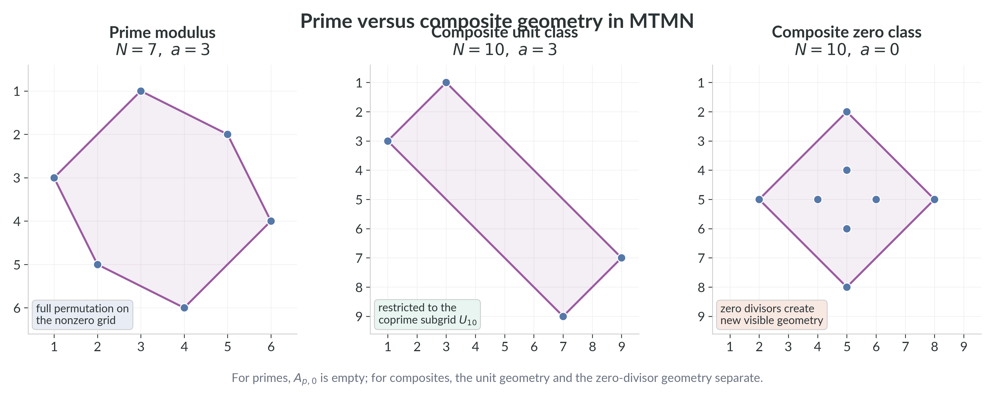
$Lattice points of $A_{7,2}$ and their convex hull. The blue dots are the lattice points satisfying $xy \equiv 2 \pmod{7}$, and the red boundary traces the convex hull.$

Two structural contrasts are worth isolating from the start. First, prime and composite moduli already behave differently: primes give the clean permutation-plot case on the whole nonzero grid, while composites split into a unit-side geometry and a zero-divisor geometry. Second, the border-by-border construction of the table will later turn into exact lower models: the first and second boundary layers are not arbitrary truncations, but the first residue-wise pieces of the same geometric object. The zero residue class will become the first place where the composite side admits a complete geometric description: its hull can be read exactly from the divisors of $N$.

@fig:prime-composite-intro highlights the first of these contrasts.

Prime and composite moduli already separate into different geometric regimes. Prime nonzero classes occupy the full nonzero grid, while composite moduli exhibit both a restricted coprime subgrid and a visible zero-divisor class.

These definitions already point toward a coherent exact theory. The present monograph concentrates on the parts that are theorem-bearing now: the residue-class areas, the prime/composite split, the solved zero-class geometry, the support-function framework, and the exact boundary models that lead to cubic-order growth for the total area.

The present book answers part of this program. In particular:

it defines the basic geometric language of the subject;
it gives exact values for small examples;
it proves that every $S(N,a)$ and $S(N)$ is a nonnegative integer;
it gives a sharp prime/composite criterion for the degeneracy of the zero class;
it describes the full zero-class hull exactly in terms of divisor rectangles, a divisor-envelope formula, and a hyperbolic correction identity;
it records an exact support-function formula for $S(N, a)$;
it develops an exact first-boundary model $S^{(1)}(N, a)$ and $S^{(1)}(N)$;
it develops an exact second-boundary model for odd $N$;
it proves that the total area $S(N)$ is trapped between explicit cubic lower and upper models, so $S(N)$ has cubic order of growth;
it packages the residue-area profile into a polynomial whose simplest evaluations isolate the zero class algebraically;
it proves that the boundary model already implies convergence of $$\sum_{N=4}^{\infty} \frac{1}{S(N)} \qquad \text{and} \qquad \sum_{N=4}^{\infty} \frac{N}{S(N)}$$ by comparison;
it gives a rigorous numerical enclosure for $\sum_{N=4}^{\infty} \frac{1}{S(N)}$.

The exposition that follows moves through the subject in that same order: first background and literature context, then the geometry of residue classes and the zero class, then exact support-function formulas, and finally the boundary-layer models suggested by the layer-by-layer construction.