The second-boundary model
Definition
The second boundary uses only rows and columns $2$ and $N-2$: $$B^{(2)}_{N,a} := A_{N,a} \cap \bigl((\{2, N-2\} \times \{1, \ldots, N-1\}) \cup (\{1, \ldots, N-1\} \times \{2, N-2\})\bigr).$$ Set $$S^{(2)}(N, a) := \operatorname{Area}(\operatorname{conv}(B^{(2)}_{N,a})), \qquad S^{(2)}(N) := \sum_{a=0}^{N-1} S^{(2)}(N, a).$$ Again one has the lower bound $$S^{(2)}(N, a) \leq S(N, a), \qquad S^{(2)}(N) \leq S(N).$$
From the construction viewpoint of Chapter 5, this is the residue-wise version of the second ring of the table. After the outer frame has been drawn, the next boundary layer comes from rows and columns $2$ and $N-2$; $B^{(2)}_{N,a}$ records only those second-layer cells whose entry is $a$.
In plainer language: first ignore the outer frame, then look only at the next ring in from the edge, and finally keep only the cells whose residue is $a$. The notation $B^{(2)}_{N,a}$ is just a compact way to say “the second ring of the residue class $A_{N,a}$.”
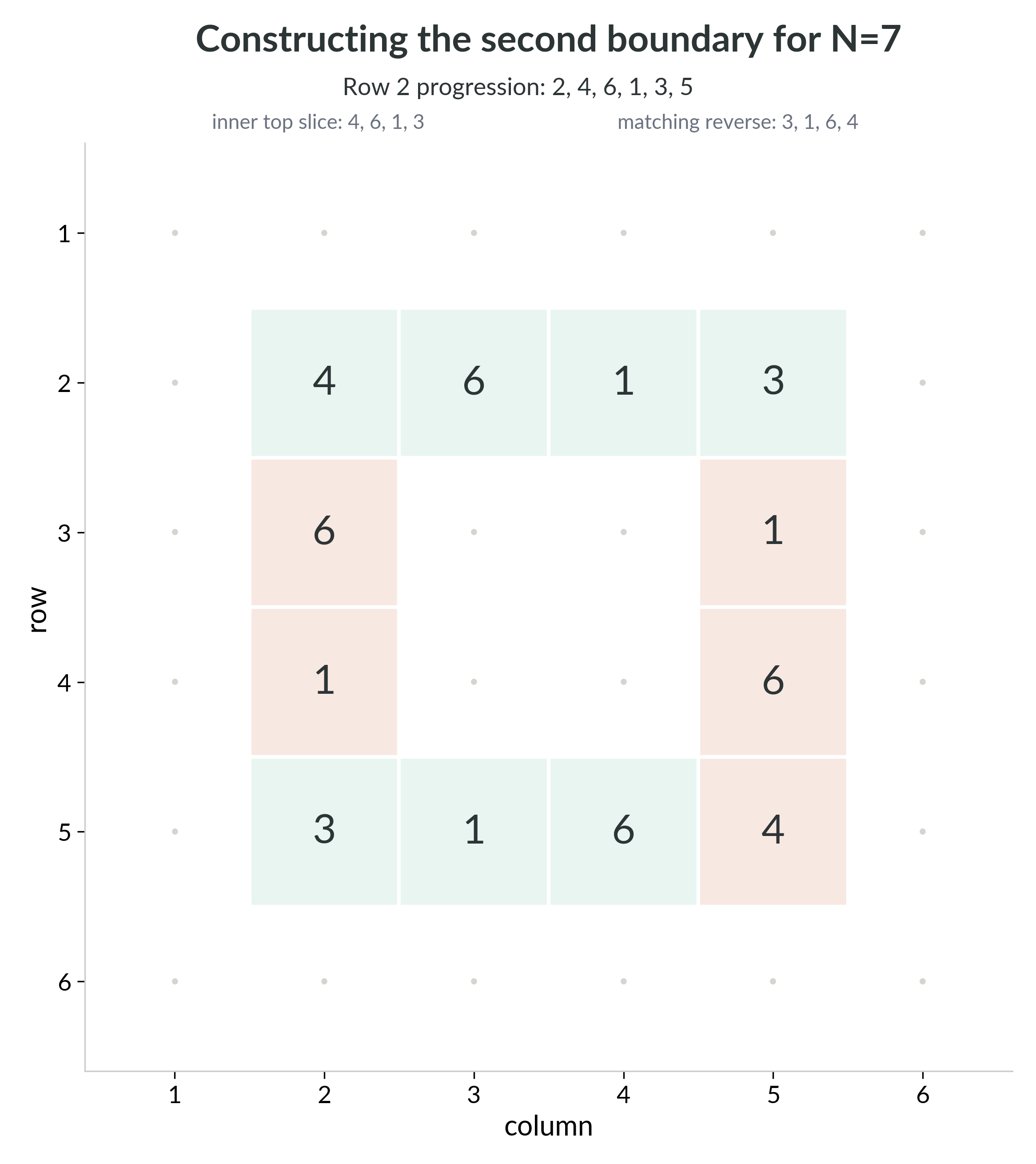
@fig:construction-layer2-n7-ch6 shows that second ring before any residue selection is made.
Exact formula for odd $N$
When $N$ is odd, the residue $2$ is invertible modulo $N$. So for each nonzero residue $a$, there is exactly one residue $b$ with $$2b \equiv a \pmod{N}.$$ The symbol $b$ is simply a convenient name for that unique hit on the second boundary. We now write it as $$b \equiv 2^{-1}a \pmod{N}, \qquad 1 \leq b \leq N-1.$$
In other words, the theorem below says: once that single number $b$ is known, the four second-boundary points are immediately determined, and so is the area of their hull.
Proof. If $x = 2$, the congruence becomes $2y \equiv a \pmod{N}$, so $y \equiv b \pmod{N}$. Since $N$ is odd, $2$ has a unique inverse modulo $N$, hence the point is $(2, b)$. Symmetrically one gets $(b, 2)$. On the rows and columns $N - 2 \equiv -2 \pmod{N}$, the congruence becomes $-2y \equiv a \pmod{N}$, hence $y \equiv N - b \pmod{N}$, producing the other two points.
Now apply the linear change of coordinates $$u = x + y, \qquad v = x - y.$$ Its Jacobian determinant has absolute value $2$, so area in $(x,y)$-space equals one half the area in $(u,v)$-space. The four points become the corners of the rectangle with $$u \in \{b+2,\; 2N - b - 2\}, \qquad v \in \{\pm(b-2)\}.$$ Therefore the rectangle in $(u,v)$-space has side lengths $$2|N - b - 2|, \qquad 2|b - 2|.$$ Dividing by $2$ gives the area in $(x,y)$-space: $$S^{(2)}(N, a) = \frac{1}{2} \cdot 2|N - b - 2| \cdot 2|b - 2| = 2|b - 2|\,|N - b - 2|.$$ □
For the zero residue, this theorem gives $S^{(2)}(N,0)=0$ for every odd $N$. That does not mean the full zero class is degenerate. Chapter 5 shows that for every odd composite modulus $N>4$, the full hull of $A_{N,0}$ still has positive area. The second boundary misses that geometry because the divisor-driven zero class lives deeper in the table than the single layer $x,y \in \{2,N-2\}$.
Proof. As $a$ runs over $1, \ldots, N-1$, so does $b \equiv 2^{-1}a \pmod{N}$. Hence $$S^{(2)}(N) = \sum_{b=1}^{N-1} 2\,|b-2|\,|N-b-2|.$$ For odd $N$, the absolute values simplify piecewise: $$S^{(2)}(N) = 2(N-3) + 2(N-3) + \sum_{b=3}^{N-3} 2(b-2)(N-b-2).$$ Evaluating the quadratic sum gives $$S^{(2)}(N) = \frac{(N-3)(N^2 - 9N + 32)}{3}.$$ A direct expansion verifies the identity. □
Geometric comparison
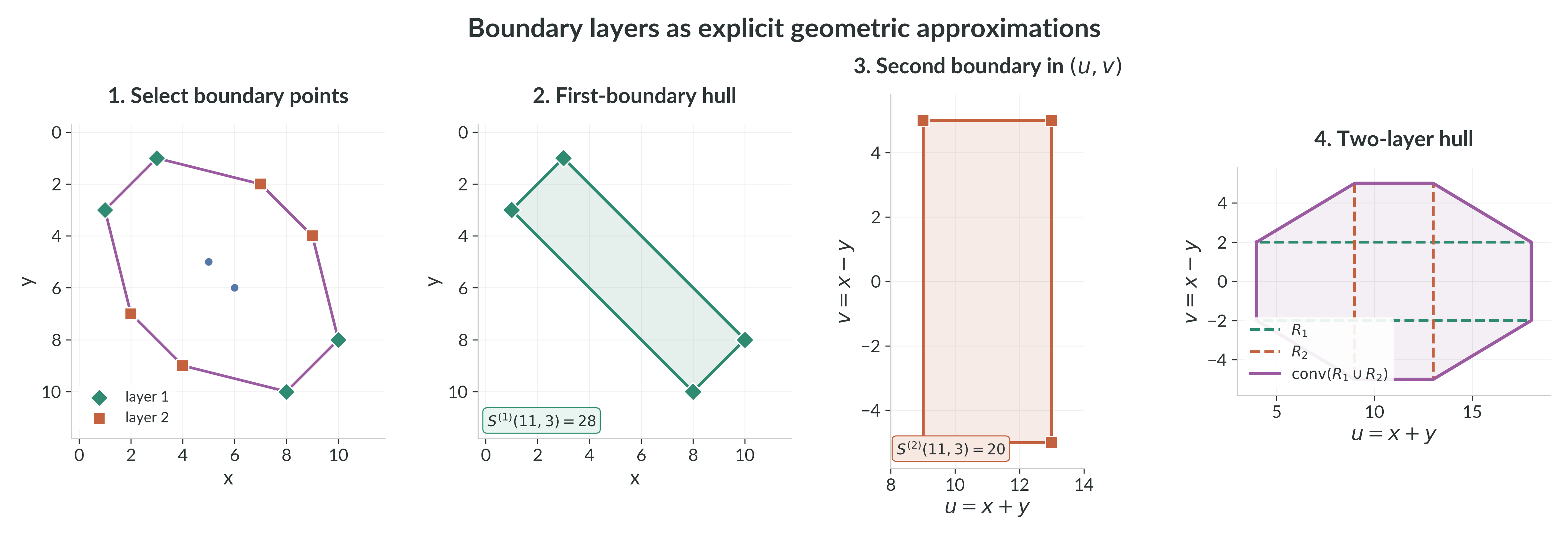
@fig:boundary-model-pipeline packages the whole boundary program for one residue class: select the first two layers inside $A_{N,a}$, identify the first-boundary hull in $(x,y)$, pass to rectangles in $(u,v)$, and then take the hull of the first two layers together.
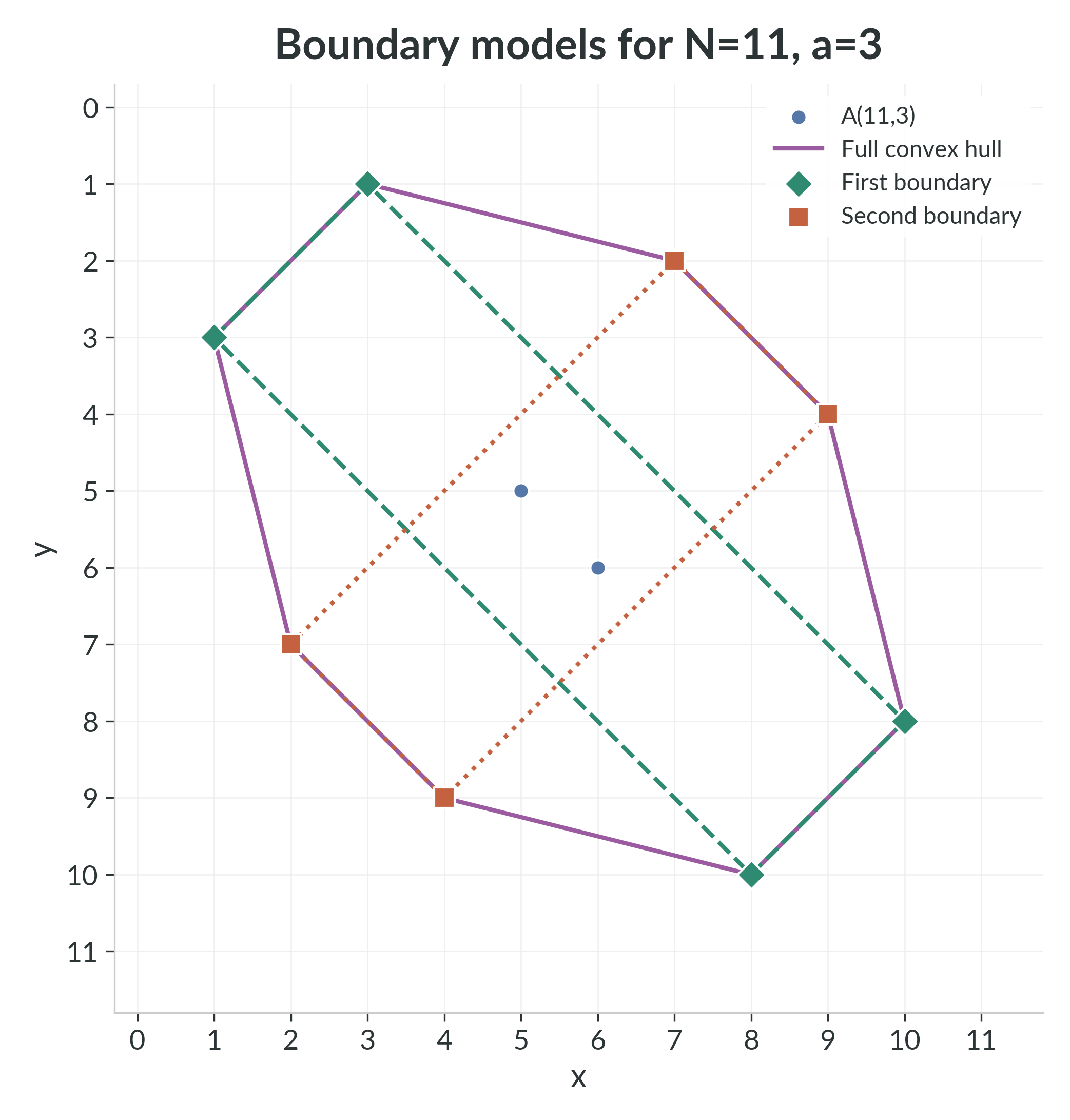
@fig:residue-class-n11-a3 compares the full residue set with the first- and second-boundary models for one sample residue class.
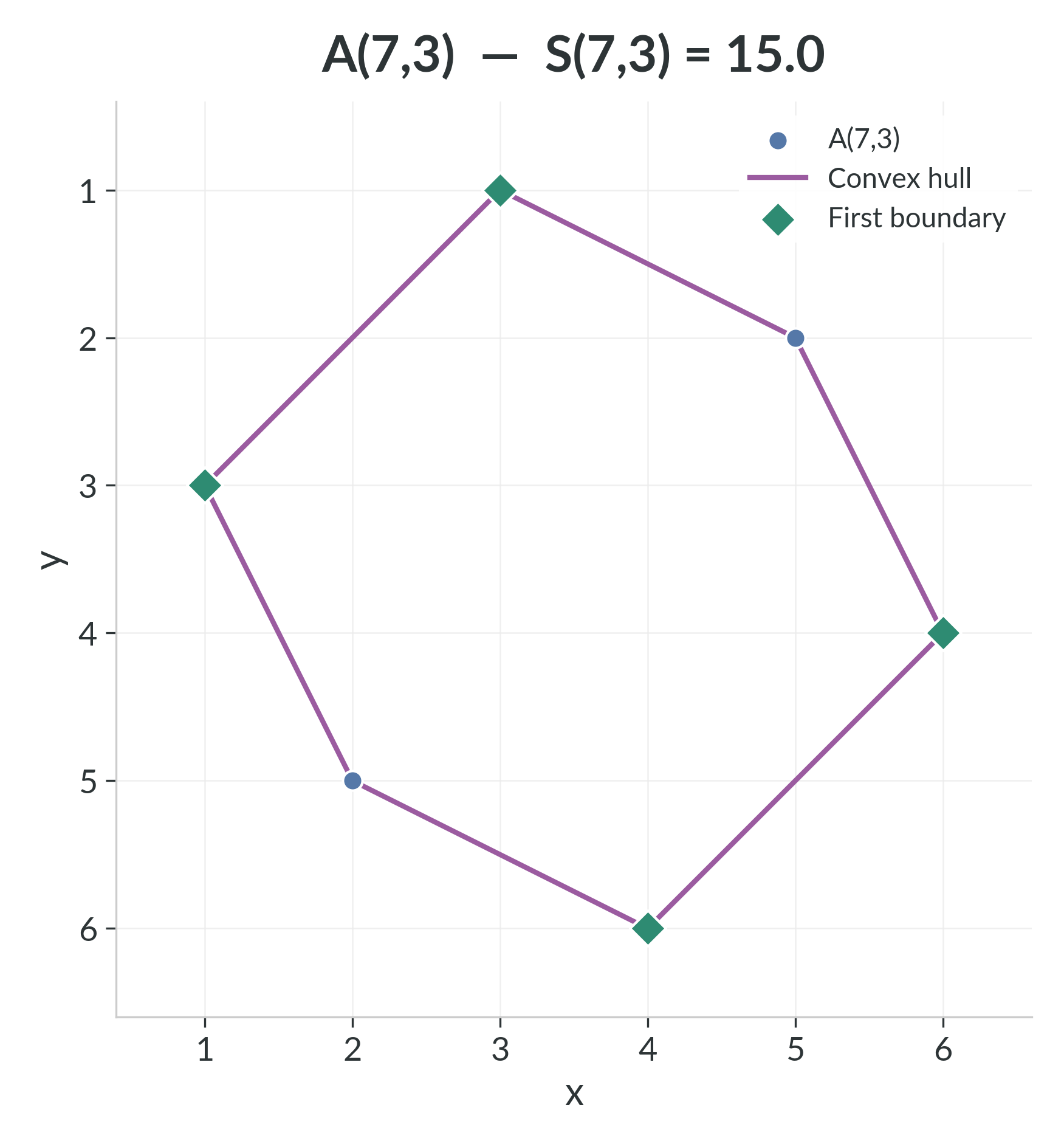
As a further illustration, @fig:residue-class-n7-a3 shows a single residue class for $N = 7$, $a = 3$ with both its hull and boundary points marked.