The first-boundary model
Definition
The first boundary, or outer frame, of the table is the union of the first row, last row, first column, and last column. Define $$B^{(1)}_{N,a} := A_{N,a} \cap \bigl((\{1, N-1\} \times \{1, \ldots, N-1\}) \cup (\{1, \ldots, N-1\} \times \{1, N-1\})\bigr).$$ Set $$S^{(1)}(N, a) := \operatorname{Area}(\operatorname{conv}(B^{(1)}_{N,a})), \qquad S^{(1)}(N) := \sum_{a=0}^{N-1} S^{(1)}(N, a).$$ By construction, $$B^{(1)}_{N,a} \subseteq A_{N,a}, \qquad S^{(1)}(N, a) \leq S(N, a), \qquad S^{(1)}(N) \leq S(N).$$ Thus $S^{(1)}$ is an exact lower-bound model.
From the layer-by-layer drawing viewpoint of Chapter 5, this is the residue-wise version of the first ring of the table. One first draws the full outer frame of MTMN; then $B^{(1)}_{N,a}$ keeps only those outer-frame cells whose entry is the residue $a$. The key point is that the model is not an arbitrary truncation. It is the first geometric approximation already forced on us by the border-by-border construction of the table itself.
Exact shape of the first boundary
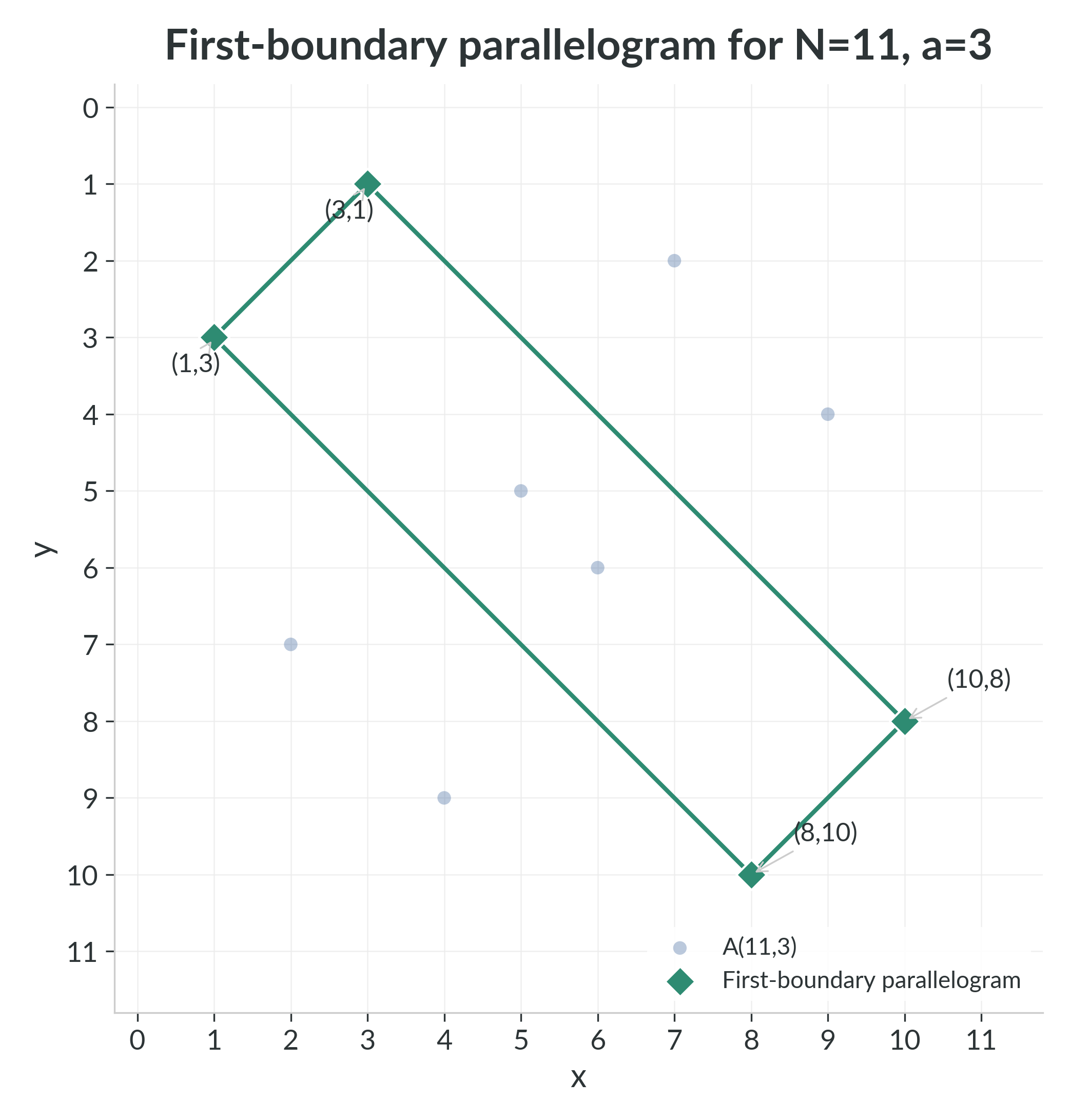
Proof. On the first row $x = 1$, the congruence $xy \equiv a \pmod{N}$ becomes $y \equiv a \pmod{N}$, so the boundary point is $(1, a)$. On the first column the point is $(a, 1)$. On the last row $x = N - 1 \equiv -1 \pmod{N}$, so $-y \equiv a \pmod{N}$, hence $y \equiv N - a \pmod{N}$, giving $(N-1, N-a)$. Similarly one gets $(N-a, N-1)$ on the last column.
The oriented area of the parallelogram spanned by the vectors $$(a, 1) - (1, a) = (a-1, 1-a)$$ and $$(N-1, N-a) - (1, a) = (N-2, N-2a)$$ is $$\left|\det\begin{pmatrix} a-1 & N-2 \\ 1-a & N-2a \end{pmatrix}\right| = 2(a-1)(N-a-1),$$ which is therefore the hull area. □
The identity $S^{(1)}(N,0)=0$ should not be confused with the full zero-class geometry. Chapter 5 shows that for every composite modulus $N>4$, the full zero-class hull has positive area. What vanishes here is only the contribution from the outer frame: the zero-divisor geometry of $A_{N,0}$ is an interior phenomenon rather than a first-boundary one.
@fig:first-boundary-parallelogram illustrates the four boundary points and their parallelogram for a specific example.
Total first-boundary sum
Proof. Using the exact first-boundary formula above, $$S^{(1)}(N) = \sum_{a=1}^{N-1} 2(a-1)(N-a-1).$$ Set $b = a - 1$, so $b = 0, 1, \ldots, N-2$. Then $$S^{(1)}(N) = 2 \sum_{b=0}^{N-2} b\bigl((N-2) - b\bigr).$$ Let $m = N - 2$. Using $$\sum_{b=0}^{m} b = \frac{m(m+1)}{2}, \qquad \sum_{b=0}^{m} b^2 = \frac{m(m+1)(2m+1)}{6},$$ we obtain $$S^{(1)}(N) = 2\left(m \cdot \frac{m(m+1)}{2} - \frac{m(m+1)(2m+1)}{6}\right) = \frac{m(m+1)(m-1)}{3},$$ which is exactly $$\frac{(N-3)(N-2)(N-1)}{3}.$$ □
The cubic scale of the total area
Recall that $S(N,a)$ is the convex-hull area of the residue class $A_{N,a}$, and that $$ S(N) = \sum_{a=0}^{N-1} S(N,a). $$ The exact first-boundary formula already forces a genuine global growth law for this total. The point is not only that one gets matching exponents after a squeeze. The statement below says that the accumulated hull area of all residue classes cannot collapse below cubic order, even though individual classes may be sparse, degenerate, or arithmetically irregular.
Proof. The lower bound is immediate from the exact lower-model inequality $$ S^{(1)}(N) \leq S(N) $$ together with the total first-boundary formula just proved. For the upper bound, fix a residue $a$. The whole set $A_{N,a}$ lies in the square $$ [1,N-1] \times [1,N-1], $$ whose area is $(N-2)^2$. Hence $\operatorname{conv}(A_{N,a})$ also lies in that square, so $$ S(N,a) \leq (N-2)^2. $$ Summing over the $N$ residue classes gives $$ S(N) \leq N(N-2)^2. $$ □
This makes $N^3$ the right first scale for the total area. There are $N$ residue classes, each class lives in a box of quadratic area scale, and summing such contributions naturally suggests a cubic total. But that is only a scale heuristic, not a proof. A large point set can still have a thin or degenerate hull, arithmetic collisions can force strong nonuniformity, and zero-divisor structure can distort the geometry from one residue to the next. The theorem matters precisely because it shows that these local irregularities do not destroy cubic growth in the aggregate.
One conceptual clarification is worth making explicit. All of the hulls $\operatorname{conv}(A_{N,a})$ lie in the same ambient square, but $S(N)$ is the sum of their areas, not the area of their union. So there is no contradiction between a quadratic Euclidean window and a cubic total: the same square is being counted once for each residue label.
The sharp cubic question
Once the exponent is fixed, the next question is the leading constant. The exact computations now available point consistently to the sharper asymptotic $$ S(N) \sim N^3. $$ Equivalently, one asks whether $$ \frac{S(N)}{N^3} \to 1 $$ as $N \to \infty$.
\textbf{Conjecture (sharp cubic asymptotic).} As $N \to \infty$, $$ S(N) \sim N^3. $$
Representative exact values are:
| $N$ | $S(N)/N^3$ |
|---|---|
| $1000$ | $0.97073535$ |
| $2000$ | $0.98325402$ |
| $3000$ | $0.98725631$ |
| $5000$ | $0.99214422$ |
These finite computations do not prove the conjecture, but they support it strongly. A related diagnostic points in the same direction: because $$ S^{(1)}(N) = \frac{(N-3)(N-2)(N-1)}{3} \sim \frac{N^3}{3}, $$ the conjecture $S(N)\sim N^3$ would imply $$ \frac{S(N)}{S^{(1)}(N)} \to 3. $$ The exact data is consistent with that drift as well.
The first-boundary model is especially revealing in this light. One explicit geometric layer already contributes a full cubic amount: $$ S^{(1)}(N) \sim \frac{N^3}{3}. $$ So if the conjecture $S(N)\sim N^3$ is true, then the outer frame is not the whole story but the first explicit third of a much fuller cubic phenomenon.
The deficiency
Once $N^3$ is recognized as the right main scale, the natural second-order object is not $S(N)$ itself but its missing area: $$ D(N) := N^3 - S(N). $$ The sharp cubic conjecture is equivalent to the statement $$ D(N) = o(N^3). $$ that is, $$ \frac{D(N)}{N^3} \to 0. $$ In that form the problem changes character. One no longer asks whether the total area grows cubically; that is already settled. One asks how much of the cubic budget is lost, why it is lost, and how that loss is distributed across residue classes.
Even the crude box cap shows that some deficit is unavoidable. Since $$ S(N) \leq N(N-2)^2 = N^3 - 4N^2 + 4N, $$ one always has $$ D(N) \geq 4N^2 - 4N. $$ So the deficiency is not expected to vanish. The real question is whether it is smaller than the cubic main term, and how sharply one can describe it. This is where the subtlety of the problem seems to live: in which points become actual hull vertices, which boundary layers dominate, and how the missing area aggregates across the residue families.
Global series consequences
The same asymptotic picture also organizes the two most natural global series formed from $S(N)$. The reciprocal series is the main one. A weighted companion reflects the same large-$N$ geometry through a slower-decaying lens, but it remains secondary to the area problem itself.
The reciprocal series
Once the total area sum $S(N)$ has been introduced, it is natural to ask whether varying the modulus leaves behind any single global quantity. The simplest one is obtained by taking reciprocals and summing over all moduli: $$ C := \sum_{N=4}^{\infty} \frac{1}{S(N)}. $$ This series gives the greatest weight to small moduli, where the total area is smallest, and discounts the larger moduli according to how quickly $S(N)$ grows. So two immediate questions arise: does the series converge, and if it does, can one say anything exact about its value?
The first-boundary model already answers the analogous question completely, because $S^{(1)}(N)$ is an explicit cubic polynomial. That exact model then becomes a comparison tool for the full series.
Proof. By the total first-boundary formula just proved, $$\frac{1}{S^{(1)}(N)} = \frac{3}{(N-3)(N-2)(N-1)}.$$ Let $k = N - 3$. Then $k \geq 1$ and $$\sum_{N=4}^{\infty} \frac{1}{S^{(1)}(N)} = \sum_{k=1}^{\infty} \frac{3}{k(k+1)(k+2)}.$$ Using the telescoping identity $$\frac{1}{k(k+1)(k+2)} = \frac{1}{2}\left(\frac{1}{k(k+1)} - \frac{1}{(k+1)(k+2)}\right),$$ we get $$\sum_{k=1}^{M} \frac{3}{k(k+1)(k+2)} = \frac{3}{2} \sum_{k=1}^{M}\left(\frac{1}{k(k+1)} - \frac{1}{(k+1)(k+2)}\right) = \frac{3}{2}\left(\frac{1}{2} - \frac{1}{(M+1)(M+2)}\right).$$ Letting $M \to \infty$ gives $3/4$. □
Proof. By construction $S(N) \geq S^{(1)}(N)$ for every $N$, so the total first-boundary formula gives $$ 0 \leq \frac{1}{S(N)} \leq \frac{1}{S^{(1)}(N)} = \frac{3}{(N-3)(N-2)(N-1)}. $$ The right-hand side is summable by the theorem above, so the full series converges by comparison. □
Proof. The proof of the theorem above already gives the exact partial-sum identity $$ \sum_{N=4}^{M} \frac{1}{S^{(1)}(N)} = \frac{3}{4} - \frac{3}{2(M-2)(M-1)}. $$ Subtracting this from the total value $3/4$ yields the stated tail formula. □
The point of the tail formula is that it immediately turns any finite exact computation of the values $S(N)$ into a rigorous interval for the full constant $C$.
Proof. Since all terms are nonnegative, $$ 0 \leq C - P_M = \sum_{N=M+1}^{\infty} \frac{1}{S(N)}. $$ Also $S(N) \geq S^{(1)}(N)$ for every $N$, so $$ \sum_{N=M+1}^{\infty} \frac{1}{S(N)} \leq \sum_{N=M+1}^{\infty} \frac{1}{S^{(1)}(N)}. $$ Apply the tail formula above. □
Proof. The displayed partial sum is the output of an exact integer computation of the finitely many values $S(N)$ for $4 \leq N \leq 2000$. Apply the preceding corollary with $M=2000$. The tail contribution is bounded by $$ \frac{3}{2(1998)(1999)} = 0.000000375563156954, $$ which gives the stated interval after addition. □
The width of this interval is below $4 \times 10^{-7}$. So the reciprocal constant is already sharply localized numerically, even though no symbolic formula is known.
From the cubic bounds developed above, the significance of the reciprocal series is clear. The first-boundary comparison already gives the correct decay scale for the tail, $$ \sum_{N=M+1}^{\infty} \frac{1}{S(N)} = O(M^{-2}), $$ so the series $$ C=\sum_{N=4}^{\infty}\frac{1}{S(N)} $$ is not only convergent but quantitatively well controlled. Computation together with the exact tail bound therefore yields a rigorous enclosure for $C$ and makes the reciprocal series a genuine global invariant attached to the area theory.
A weighted companion
The same large-$N$ picture has a natural weighted companion: $$ W := \sum_{N=4}^{\infty} \frac{N}{S(N)}. $$ Because the extra factor $N$ removes one power of the cubic growth, this series is more sensitive to the sharp asymptotic while still remaining summable.
Proof. By the total first-boundary formula, $$\frac{N}{S^{(1)}(N)} = \frac{3N}{(N-3)(N-2)(N-1)}.$$ Let $k = N-3$. Then $k \geq 1$ and $$\sum_{N=4}^{\infty} \frac{N}{S^{(1)}(N)} = \sum_{k=1}^{\infty} \frac{3(k+3)}{k(k+1)(k+2)}.$$ Partial fractions give $$\frac{3(k+3)}{k(k+1)(k+2)} = \frac{9}{2k} - \frac{6}{k+1} + \frac{3}{2(k+2)}.$$ Therefore $$\sum_{k=1}^{M} \frac{3(k+3)}{k(k+1)(k+2)} = \frac{9}{2}H_M - 6H_{M+1} + 6 + \frac{3}{2}H_{M+2} - \frac{9}{4},$$ where $H_M$ is the $M$-th harmonic number. Since $$H_{M+1} = H_M + \frac{1}{M+1}, \qquad H_{M+2} = H_M + \frac{1}{M+1} + \frac{1}{M+2},$$ the harmonic terms cancel and one gets $$\sum_{k=1}^{M} \frac{3(k+3)}{k(k+1)(k+2)} = \frac{15}{4} - \frac{9}{2(M+1)} + \frac{3}{2(M+2)}.$$ Letting $M \to \infty$ gives $15/4$. □
If the conjectural asymptotic $S(N)\sim N^3$ is true, then $$ \frac{N}{S(N)} \sim \frac{1}{N^2}, $$ so the weighted tail should satisfy $$ \sum_{N=M+1}^{\infty} \frac{N}{S(N)} \sim \frac{1}{M}. $$ Thus the weighted series is useful as a secondary diagnostic of the same cubic picture. Exact computation together with the first-boundary comparison currently places its full constant in a narrow rigorous interval just above $3.001$, but the point here is not the decimal expansion itself. The main point is that the weighted series, like the reciprocal series, reflects the same unresolved asymptotic geometry of $S(N)$.