The basic geometry of MTMN

Definition of the residue classes

For each residue $a$, the set $A_{N,a}$ is a finite subset of the square lattice. The collection $$\{A_{N,0},\; A_{N,1},\; \ldots,\; A_{N,N-1}\}$$ partitions the entire lattice square $\{1, \ldots, N-1\}^2$ according to the residue of the product $xy$ modulo $N$.

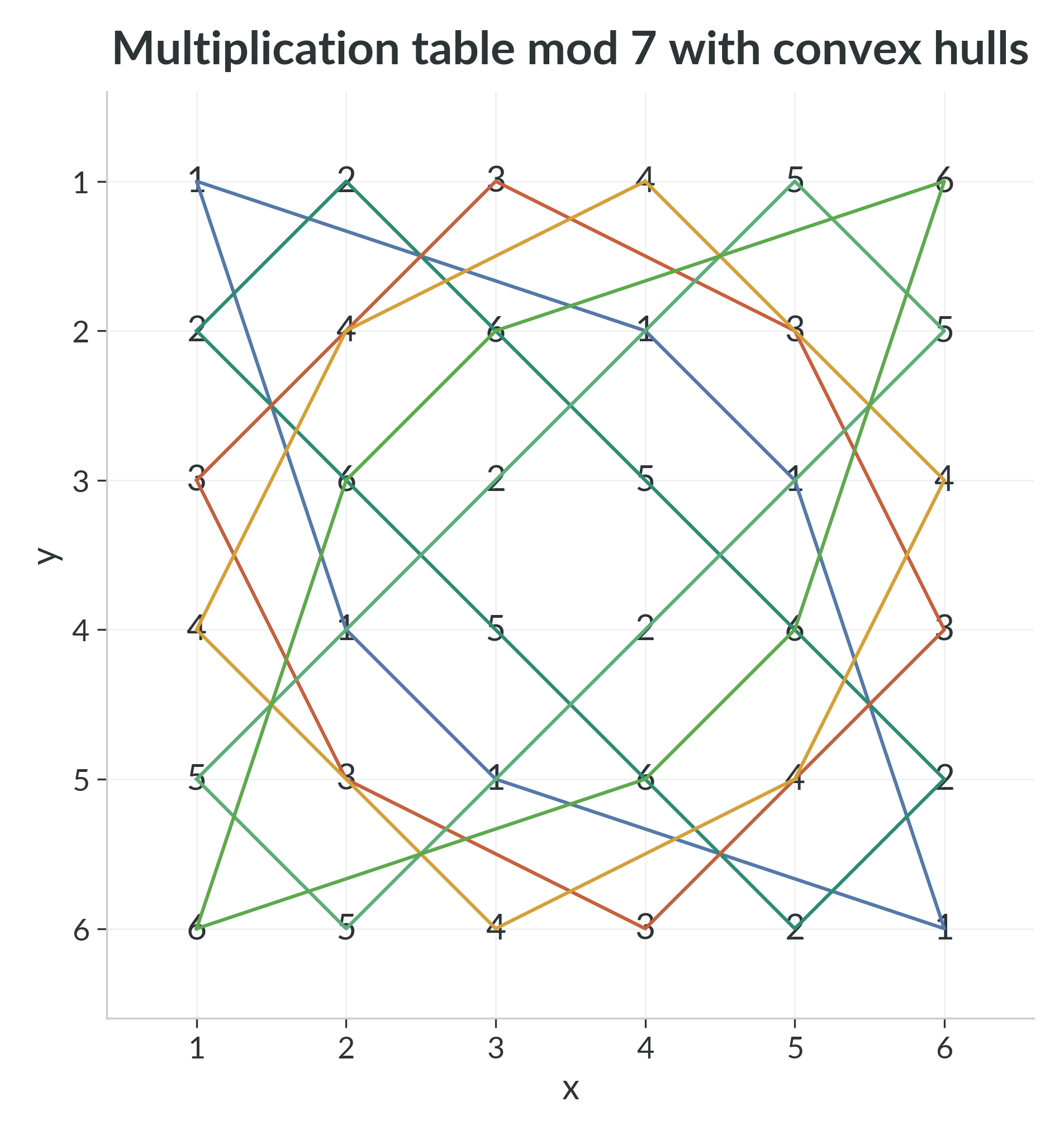
@fig:mtmn-grid-n7 shows the full multiplication table modulo $7$: each cell displays the residue $xy \bmod 7$, and the convex hull of every residue class is overlaid.

Explore interactively

Connecting Residue Points

Before one passes to convex hulls, there is already a natural straight-line object attached to a residue class. The informal picture is what one might casually call "connect the dots," but here we will use the more precise phrase Connecting Residue Points.

For a fixed residue class $A_{N,a}$, join every pair of points in $A_{N,a}$ by a straight segment and take the union of all those segments: $$ L_{N,a} := \bigcup_{p,q \in A_{N,a}} [p,q]. $$ Thus $$ A_{N,a} \subseteq L_{N,a} \subseteq \operatorname{conv}(A_{N,a}). $$

Read from left to right, this is a chain from the smallest object to the largest one in the set-theoretic sense of containment: the discrete residue set $A_{N,a}$, then the union of all connecting segments $L_{N,a}$, and finally the full convex hull. Here the symbol $\subseteq$ allows equality, just as $\leq$ allows equality for numbers. The word "larger" is therefore about inclusion, not about visible richness of structure.

In fact, the middle object can carry more geometric detail than the hull, because the hull fills everything inside its outer boundary. Here "outer envelope" means exactly that outer wrapper. For instance, if three points are non-collinear, meaning that they do not all lie on one straight line, then Connecting Residue Points gives only the three edges of the triangle, while the convex hull also contains the interior.

This book will still focus mainly on convex hulls and their areas, but naming this intermediate layer now makes its purpose explicit: it records the finer segment structure that is discarded when one passes from the residue set to its hull.

\begin{center} \begin{MTMNFigureCard} \centering \textbf{A running picture: $A_{5,2}$}\par\medskip \begin{minipage}[t]{0.23\linewidth}\centering {\scriptsize\textbf{1. Empty grid}}\par\smallskip \includegraphics[width=\linewidth]{figures/crp_a52_stage1_empty.png} \end{minipage}\hfill \begin{minipage}[t]{0.23\linewidth}\centering {\scriptsize\textbf{2. Residue points}}\par\smallskip \includegraphics[width=\linewidth]{figures/crp_a52_stage2_points.png} \end{minipage}\hfill \begin{minipage}[t]{0.23\linewidth}\centering {\scriptsize\textbf{3. Convex hull}}\par\smallskip \includegraphics[width=\linewidth]{figures/crp_a52_stage3_hull.png} \end{minipage}\hfill \begin{minipage}[t]{0.23\linewidth}\centering {\scriptsize\textbf{4. Connecting segments}}\par\smallskip \includegraphics[width=\linewidth]{figures/crp_a52_stage4_segments.png} \end{minipage} \captionof{figure}{A concrete progression for $A_{5,2}$: the empty lattice window, the residue points, the convex hull, and the full Connecting Residue Points object.} \end{MTMNFigureCard} \end{center}

How to draw MTMN layer by layer

One does not need to compute every product $xy$ separately in order to draw the table. Fix a row index $k$. The $k$-th row is $$k, \; 2k, \; 3k, \; \ldots, \; (N-1)k \pmod{N},$$ so after the first entry every new value is obtained by adding $k$ modulo $N$.

Proof. Fix a column index $y$. The entry in row $N-k$ and column $y$ is $$(N-k)y \equiv k(N-y) \pmod{N}.$$ The right-hand side is exactly the entry in row $k$ and column $N-y$. Therefore the value appearing in row $N-k$ at position $y$ is the value appearing in row $k$ at the reflected position $N-y$. As $y$ runs through $1,\ldots,N-1$, the number $N-y$ runs through $N-1,\ldots,1$, so row $N-k$ is row $k$ read in reverse order.

Since the multiplication table is symmetric across the diagonal ($xy=yx$), the same reasoning applies to columns. The $k$-th boundary layer consists of the top row $k$, the bottom row $N-k$, the left column $k$, and the right column $N-k$. Hence one modular progression and its reverse determine the whole boundary ring.

For example, when $N=7$ and $k=2$, the row-$2$ progression is $$2,\;4,\;6,\;1,\;3,\;5,$$ while the row-$5$ progression is $$5,\;3,\;1,\;6,\;4,\;2,$$ which is its reverse. The second boundary layer is therefore already encoded in that one row. □

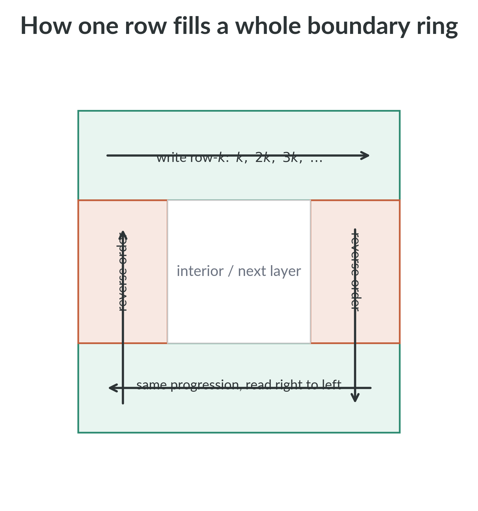
The practical rule is therefore simple. First write the row-$k$ progression across the top side of the $k$-th layer. Then continue around the same ring: the right and left sides use the reversed order, while the bottom side uses the forward order when read from right to left. In this way a single repeated-addition sequence fills an entire border.

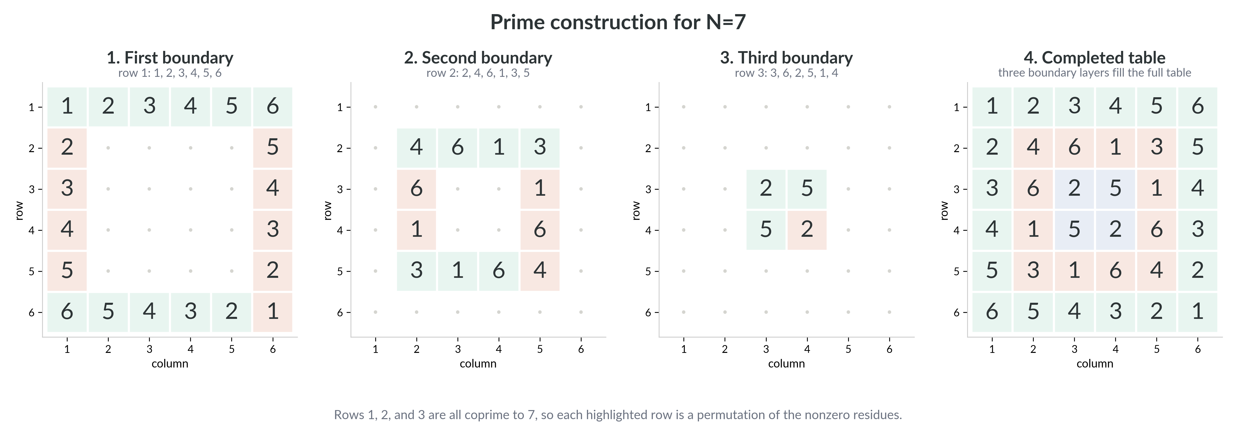
For $N = 7$, the first row gives $$1, \; 2, \; 3, \; 4, \; 5, \; 6,$$ so the first boundary is immediate. The second row gives $$2, \; 4, \; 6, \; 1, \; 3, \; 5,$$ which fills the second boundary by the same rule. The third row gives $$3, \; 6, \; 2, \; 5, \; 1, \; 4,$$ which fills the third boundary and therefore completes the table. Because the row indices $1$, $2$, and $3$ are all coprime to $7$, each of those rows is a rearrangement of the nonzero residues. The prime picture is therefore built by successive permutations.

@fig:construction-n7 shows that prime case from start to finish: first boundary, second boundary, third boundary, then the completed table. By the time the full picture is on the page, one can already see the first informal glimpse of permutation geometry: every nonzero row and every nonzero column contains each nonzero residue exactly once.

Explore interactively

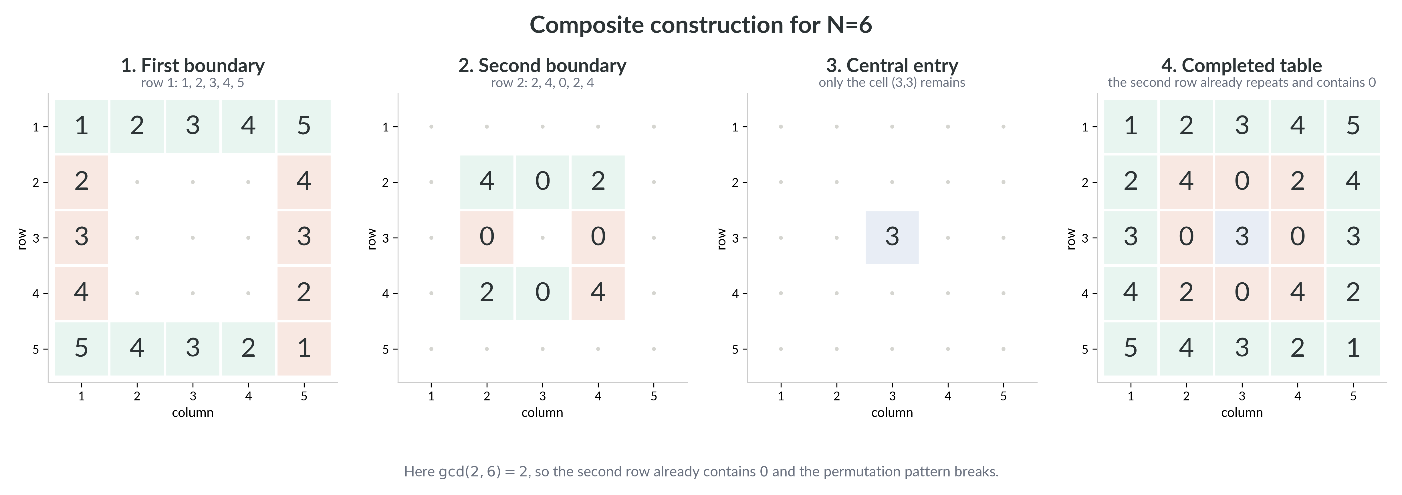
Only after the $N=7$ story is complete is it helpful to contrast it with a composite modulus. For $N=6$, the first row still gives a full nonzero progression, but the second row is $$2, \; 4, \; 0, \; 2, \; 4,$$ so repetition and a zero appear immediately on the second boundary. Here the reason is arithmetic: $2$ and $6$ share the common factor $2$, so $2 \cdot 3 \equiv 0 \pmod{6}$. Once a row or column contains $0$, it can no longer list the nonzero residues exactly once.

@fig:construction-n6 shows the same construction for $N=6$: first boundary, second boundary, the central entry, and the completed table. The procedure is unchanged, but the arithmetic is different.

Explore interactively

@fig:construction-directions isolates the directional rule around one boundary ring.

Explore interactively

This contrast isolates the key arithmetic rule. A number $k$ is coprime to $N$ if $\gcd(k,N)=1$, meaning that $k$ and $N$ share no common factor greater than $1$. Equivalently, $k$ is invertible modulo $N$: there exists some $k^{-1}$ with $k k^{-1} \equiv 1 \pmod{N}$. When $k$ is coprime to $N$, multiplication by $k$ rearranges the nonzero residues. When $k$ is not coprime to $N$, a zero appears and the permutation pattern breaks.

This border-by-border picture is more than a drawing trick. For a fixed residue $a$, one may keep only those cells on the first ring whose value is $a$; that residue-wise subset will become the first boundary model $B^{(1)}_{N,a}$. Keeping the next ring gives the second boundary model $B^{(2)}_{N,a}$. In this sense the boundary program of Chapters 7 and 8 is already visible in the construction itself: the early layers of the table are the first explicit geometric approximations to the full residue class.

Two complete first examples

Before turning to the general propositions, it is worth seeing the first prime and composite cases in full. These two moduli are small enough that one can hold the whole table, all residue classes, and the area data in view at once. They will serve as anchors for the later abstract statements.

The Case $N = 5$

Since $5$ is prime, every nonzero index is coprime to $5$, so this is the cleanest first example.

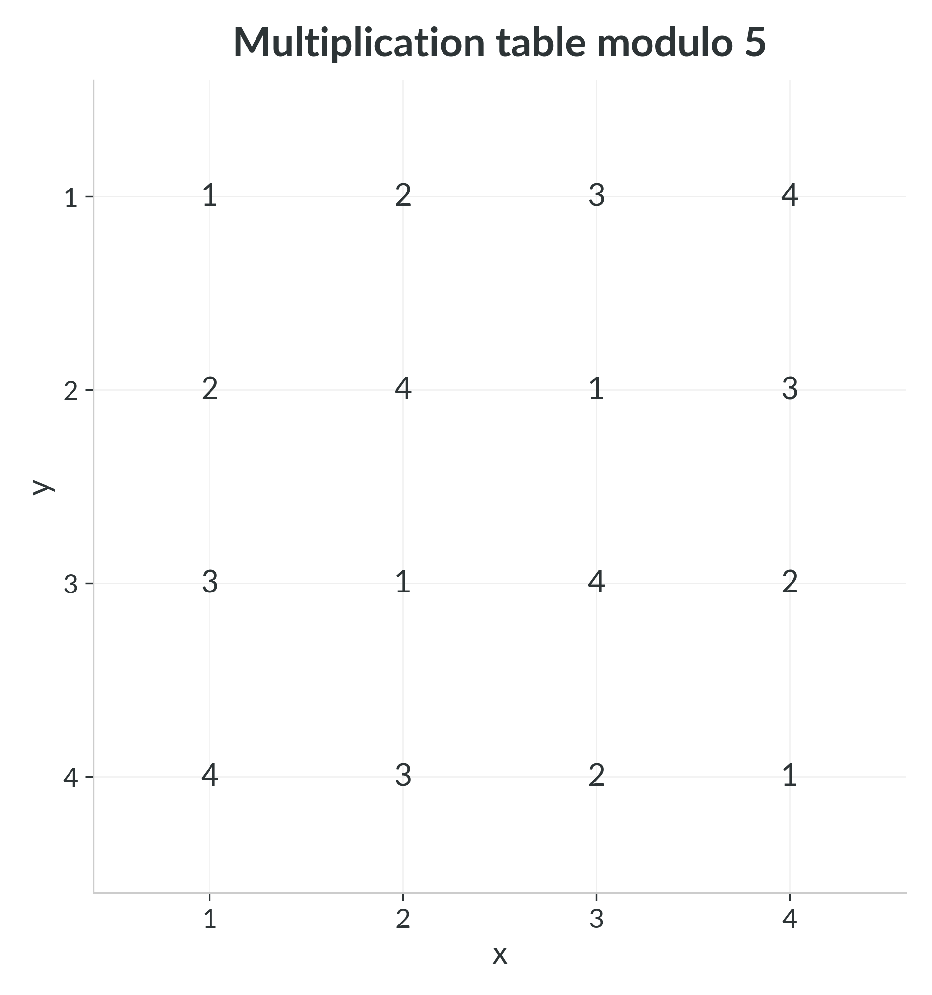
@fig:mtmn-numbers-n5 shows the raw multiplication table modulo $5$.

Explore interactively

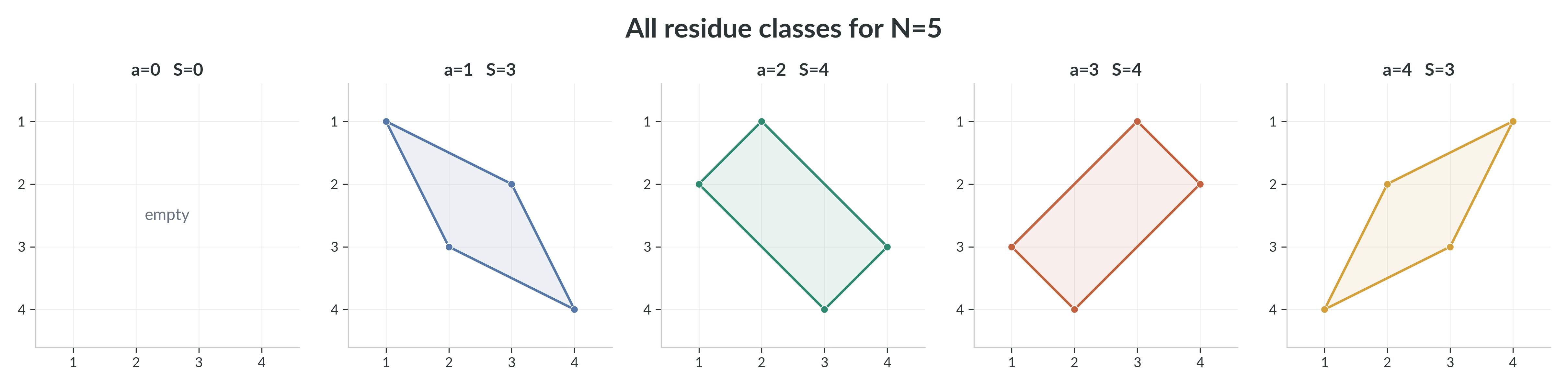
@fig:residue-classes-n5 separates the residue classes. Each panel is labeled by $a$ and by the corresponding area $S(5,a)$.

Explore interactively

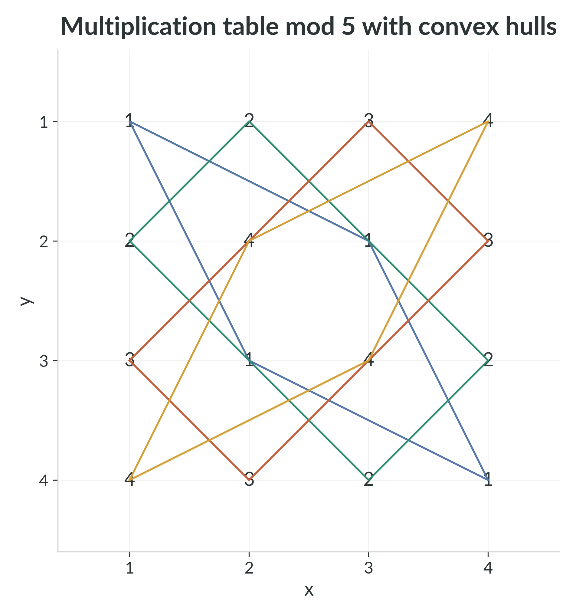
@fig:mtmn-grid-n5-ch3 overlays the nondegenerate convex hulls on the original table, so the geometry can be compared directly with the residue values.

Explore interactively

The Case $N = 6$

For $N = 6$, zero divisors already appear, so the composite case changes both the arithmetic and the geometry.

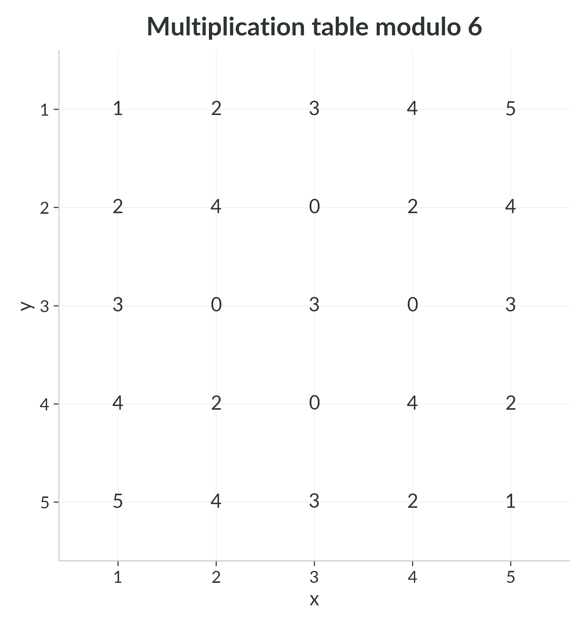
@fig:mtmn-numbers-n6 shows the raw multiplication table modulo $6$.

Explore interactively

@fig:residue-classes-n6 separates the individual residue classes. Here the zero-divisor behavior is already visible in the shapes and in the degenerate cases $S(6,1)=S(6,5)=0$.

Explore interactively

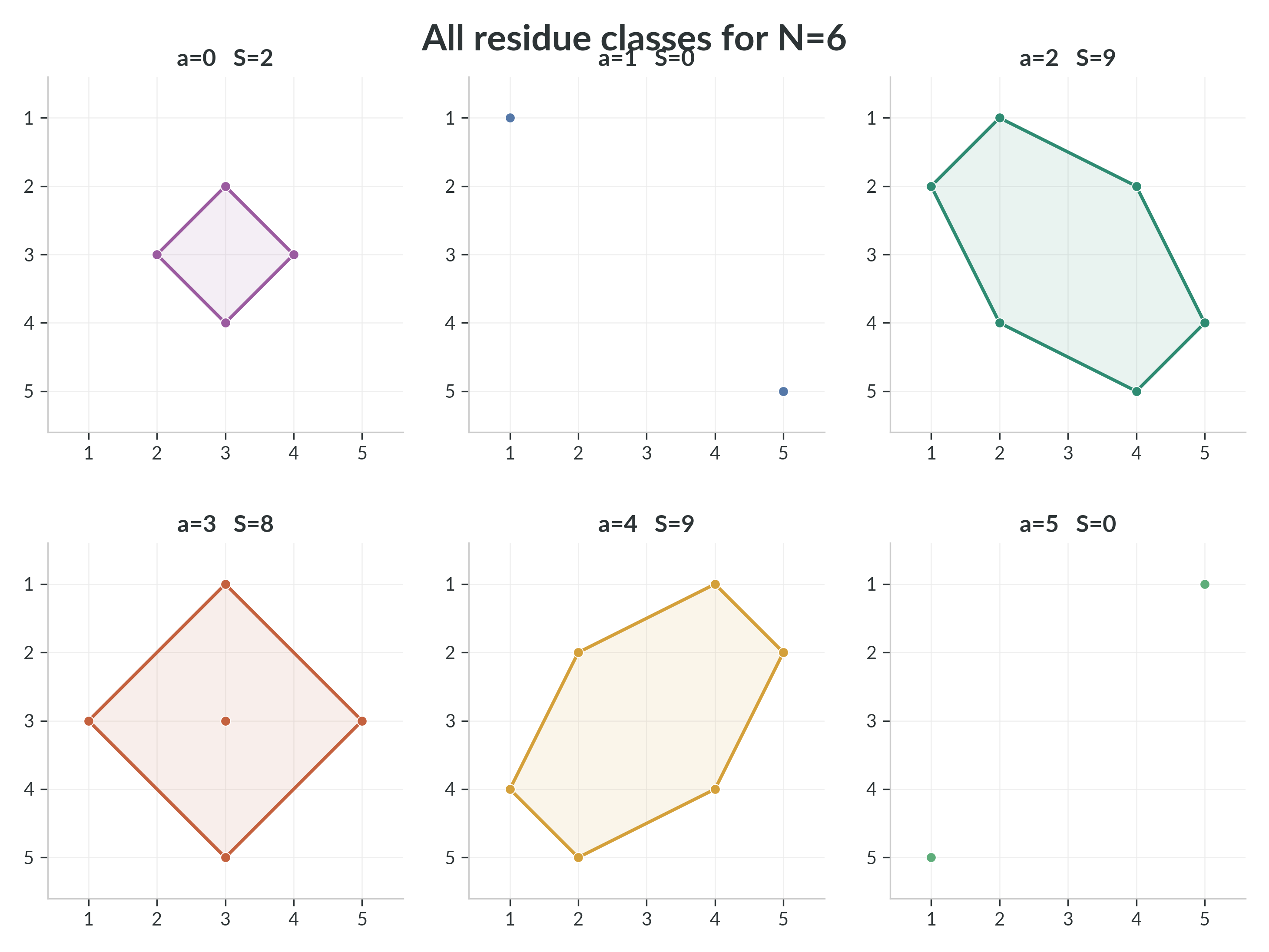
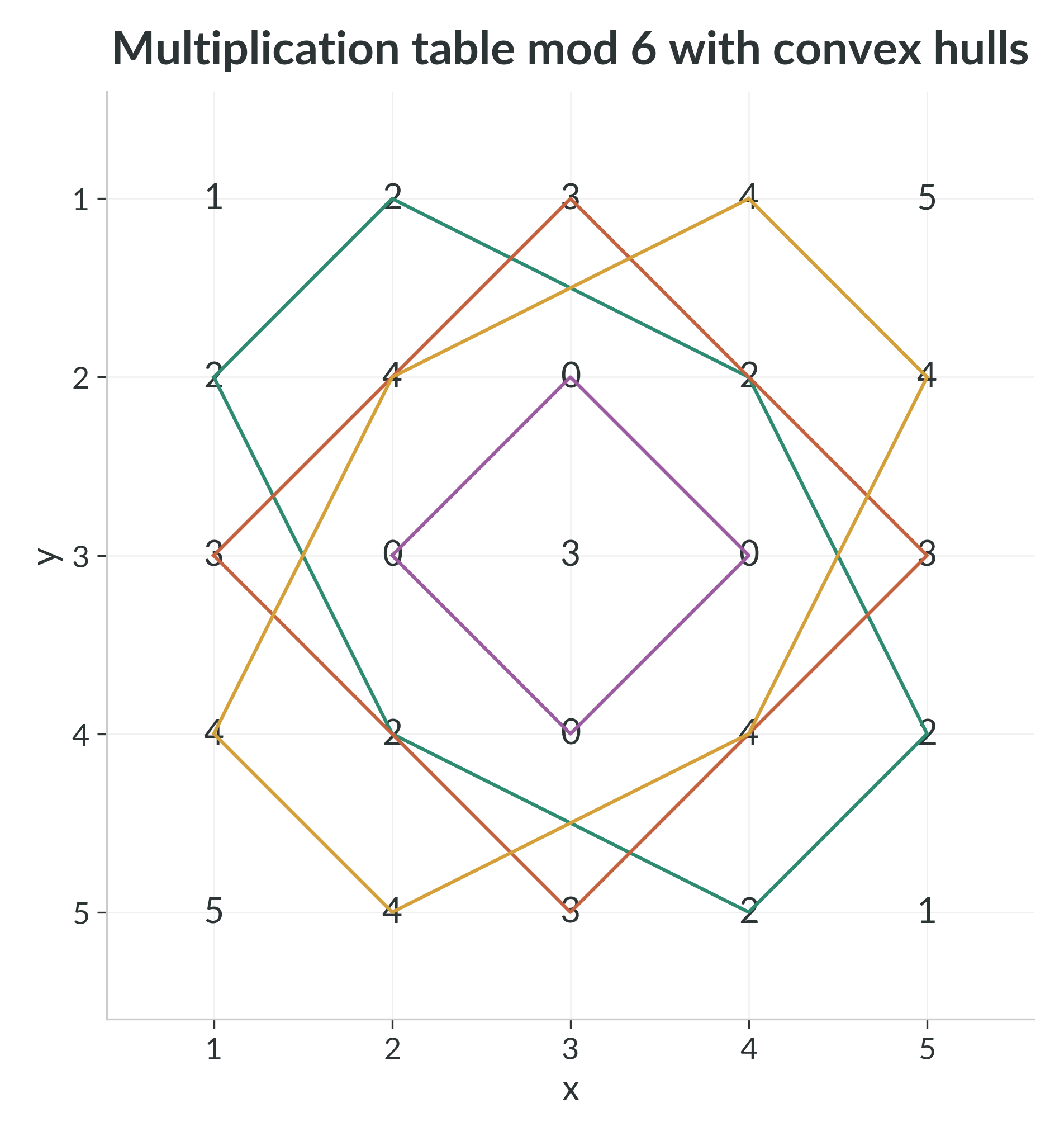
@fig:mtmn-grid-n6 overlays all nondegenerate convex hulls on the original numbers.

Explore interactively

A table of initial values

For reference, the exact totals for $4 \leq N \leq 10$ are:

A more detailed table appears in the appendix.

Euclidean symmetries of the residue classes

Proof. If $(x, y) \in A_{N,a}$, then $xy \equiv a \pmod{N}$. Since multiplication is commutative, $yx \equiv a \pmod{N}$, so $(y, x) \in A_{N,a}$. Also $$(N-x)(N-y) \equiv xy \pmod{N},$$ so $(N-x, N-y) \in A_{N,a}$ as well.

Both maps are affine maps, meaning linear transformations possibly followed by a translation. More specifically, the transpose is linear, and $(x,y)\mapsto(N-x,N-y)$ is the half-turn about the center $(N/2,N/2)$. We use the elementary fact that affine maps carry convex hulls to convex hulls, so these symmetries of the finite set $A_{N,a}$ become the corresponding symmetries of $\operatorname{conv}(A_{N,a})$. □

Proof. The reflection $$(x, y) \mapsto (x, N-y)$$ preserves Euclidean area and satisfies $$xy \equiv a \pmod{N} \implies x(N-y) \equiv -xy \equiv -a \pmod{N}.$$ Hence it carries $A_{N,a}$ onto $A_{N,(-a)\bmod N}$, so the two convex hulls have equal area. For a concrete example, when $N=7$ and $a=2$, the points $$(1,2),\ (2,1),\ (5,6),\ (6,5) \in A_{7,2}$$ are reflected to $$(1,5),\ (2,6),\ (5,1),\ (6,2) \in A_{7,5}.$$ The whole residue class transforms in exactly that way, so the two hulls have equal area. □

Proof. If $\operatorname{conv}(A_{N,a})$ is degenerate (a single point or a line segment, so it has no area), then $S(N,a)=0$. Otherwise, the half-turn from Proposition~\ref{prop:mtmn-symmetries} pairs every boundary lattice point with a distinct partner, so the boundary count $B$ is even. Pick's theorem then gives $$S(N,a) = I + \frac{B}{2} - 1,$$ which is an integer since $I$ is an integer and $B$ is even. Area is nonnegative, so $S(N,a) \in \mathbb{Z}_{\ge 0}$. Summing over $a$ yields the same for $S(N)$. □

Coprimality and permutation geometry

A permutation is first a one-dimensional object: a rearrangement of a list with no repetitions. If one then plots the input $x$ against the permuted output $\pi(x)$, that same rearrangement becomes a two-dimensional scatter plot with exactly one dot in every row and every column. This is the sense in which we will use the phrase permutation plot. For the present monograph, the planar case already captures the essential idea.

Proof. Suppose first that $\gcd(k,N)=1$. Then there exists a residue $k^{-1}$ such that $$k k^{-1} \equiv 1 \pmod{N}.$$ If two entries in the $k$-th row coincide, say $$k y_1 \equiv k y_2 \pmod{N},$$ then multiplying by $k^{-1}$ gives $y_1 \equiv y_2 \pmod{N}$. Since $y_1,y_2 \in \{1,\ldots,N-1\}$, this forces $y_1=y_2$. Therefore the entries $$k,\ 2k,\ \ldots,\ (N-1)k \pmod{N}$$ are all distinct.

Next, none of those entries is $0$. Indeed, if there existed $y \in \{1,\ldots,N-1\}$ with $ky \equiv 0 \pmod{N}$, then multiplying by $k^{-1}$ would give $y \equiv 0 \pmod{N}$, impossible. So the row contains $N-1$ distinct nonzero residues, hence exactly the set $\{1,\ldots,N-1\}$.

Conversely, if $\gcd(k,N)=d>1$, then $N/d$ is an integer with $1 \leq N/d \leq N-1$, and $$k \cdot \frac{N}{d} \equiv 0 \pmod{N},$$ so the row contains $0$ and therefore cannot be a permutation of the nonzero residues. The same argument applies to the column. □

Proof. Suppose $(x,y) \in A_{N,a}$, so $xy \equiv a \pmod{N}$. If $x$ shared a common factor $d>1$ with $N$, then $d$ would divide both $xy$ and $N$, hence also $a$, contradicting $\gcd(a,N)=1$. Thus every point of $A_{N,a}$ lies in a row indexed by a number coprime to $N$. The same argument shows that every point also lies in a column indexed by a number coprime to $N$.

Now fix a row index $x$ with $\gcd(x,N)=1$. By Proposition~\ref{prop:rows-columns-permute}, that row is a permutation of the nonzero residues $1,\ldots,N-1$. In particular, the residue $a$ appears exactly once in the row, so there is exactly one point of $A_{N,a}$ in it. The same argument applies to columns. Therefore, on the coprime subgrid, the residue class has exactly one point in each row and each column, which is exactly the permutation-plot property. □

The prime case is now the cleanest special case. If $N=p$ is prime, then every nonzero index is coprime to $p$. Therefore every nonzero residue class $A_{p,a}$ is a permutation plot on the whole nonzero grid. This does not solve the convex-hull problem by itself, but it shows that prime nonzero classes already come with a rigid row-and-column structure.

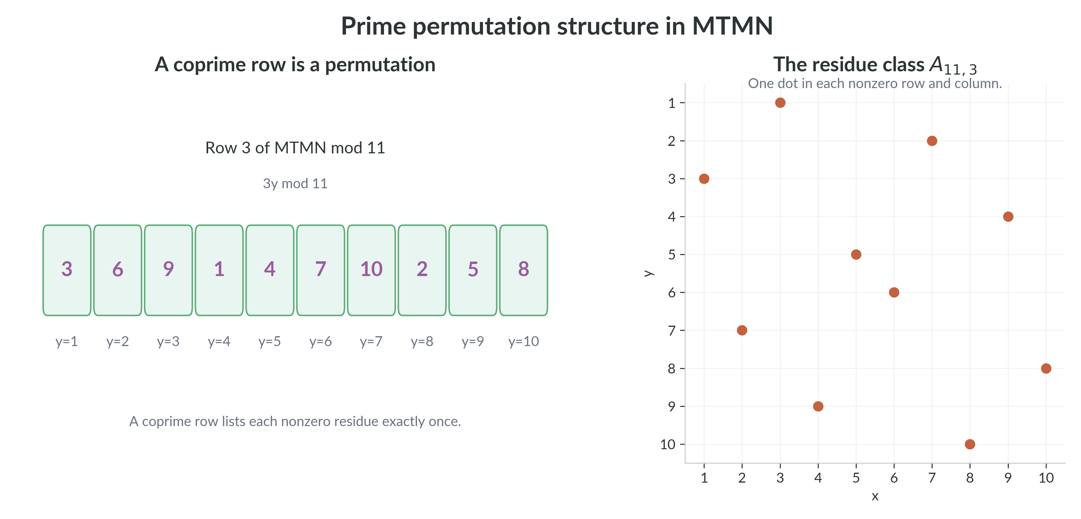
@fig:permutation-plot shows the prime example in the two ways that matter here. On the left, one coprime row of the multiplication table is read as a permutation of the nonzero residues. On the right, the residue class $A_{11,3}$ is drawn on the lattice, where the geometric content is that there is exactly one point in each nonzero row and each nonzero column.

This rigid picture also has a modern discrepancy-theoretic counterpart. Blomer, Risager, and Shparlinski study normalized inverse pairs and prove upper and lower bounds for their box, ball, and isotropic discrepancy, explicitly noting visible small-scale cellular structure and deviations from random behavior [@blomerrisagershparlinski2025]. Their setting is different from MTMN: they vary the modulus, aggregate only inverse pairs, and work on the unit side. Our setting fixes one modulus $N$, studies one residue class inside a finite lattice window, and then compares the whole residue family including zero divisors. But the geometric moral is the same. Coprime classes are not random point clouds; arithmetic imposes a rigid permutation geometry that remains visible even before one asks for exact hull formulas.

The zero class and zero-divisor geometry

The zero class and compositeness

Proof. If $p$ is prime and $1 \leq x, y \leq p-1$, then neither $x$ nor $y$ is divisible by $p$, so $xy \not\equiv 0 \pmod{p}$. Hence $A_{p,0}=\varnothing$.

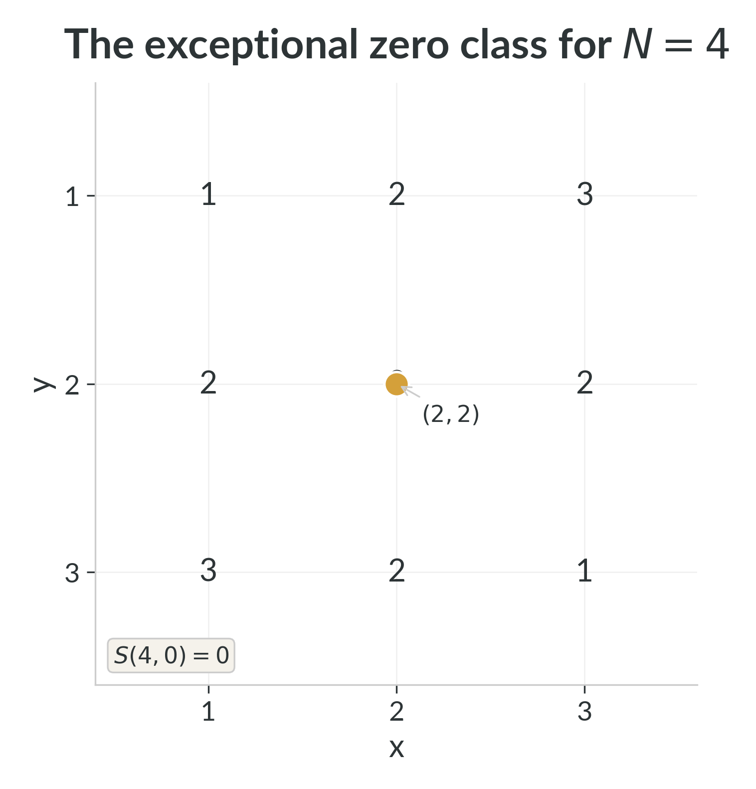
If $N$ is composite, then there exist integers $d,e$ with $1

The class $A_{N,0}$ is therefore the residue class where the same obstruction becomes most concentrated: zero divisors can multiply to $0 \pmod{N}$. This is one of the clearest differences between prime and composite moduli.

The exceptional modulus $N=4$

The point-set statement does not yet determine the geometry of the hull once the zero class becomes nonempty. The smallest composite modulus already shows the subtlety. For $N=4$ one has $$A_{4,0} = \{(2,2)\},$$ so the zero class is present but still degenerate: $$S(4,0)=0.$$ Thus nonemptiness alone does not force positive area.

@fig:zero-class-n4 marks this exceptional case directly on the $N=4$ residue grid. The lone point $(2,2)$ is present, but a single point still has zero area.

Explore interactively

When does the zero class have positive area?

Proof. If $N$ is prime, there are no zero divisors modulo $N$, so $A_{N,0}=\varnothing$ by Proposition~\ref{prop:zero-class-detects-compositeness}. Hence $S(N,0)=0$.

Now assume that $N$ is composite and $N>4$.

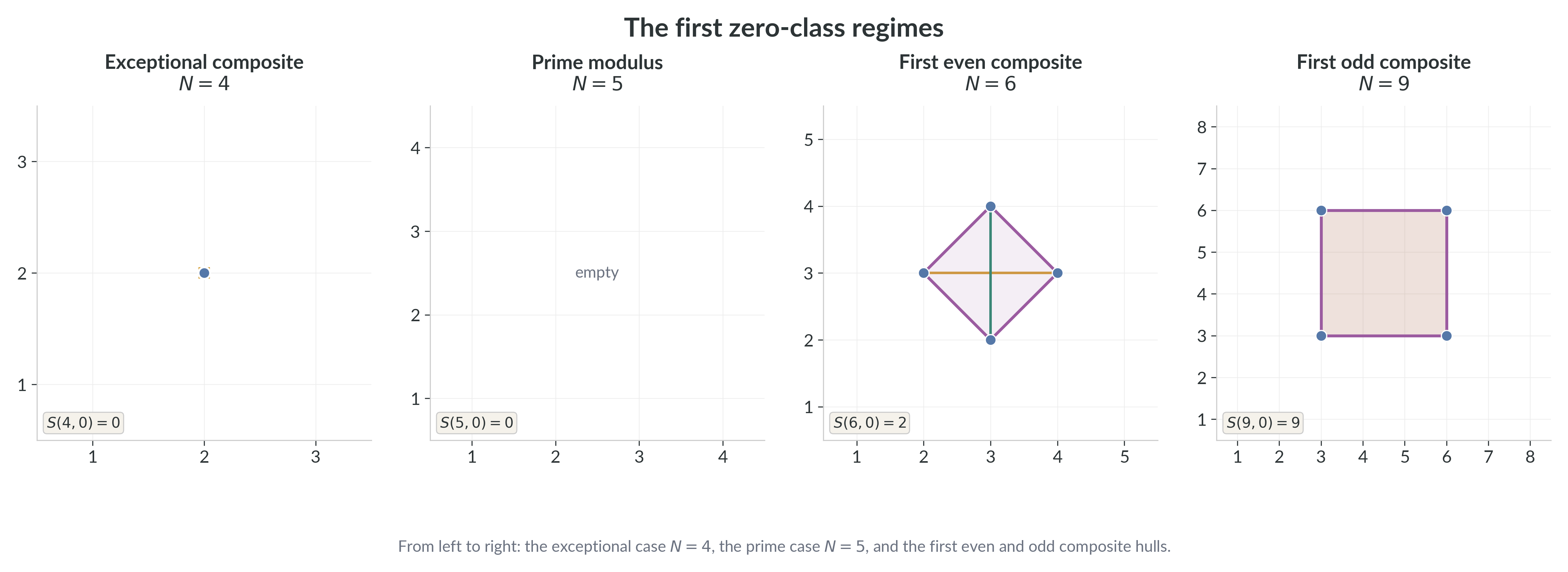
If $N$ is even, the four points $$(2,N/2), \quad (N/2,2), \quad (N-2,N/2), \quad (N/2,N-2)$$ all lie in $A_{N,0}$, since each product is divisible by $N$. They are distinct because $N>4$ implies $2 \neq N/2 \neq N-2$. These four points are the vertices of a rhombus centered at $(N/2,N/2)$, and its diagonals both have positive length. Therefore the rhombus has positive area, so $S(N,0)>0$.

If $N$ is odd composite, then there exists a proper divisor $d$ of $N$ with $10$.

Thus every composite $N>4$ satisfies $S(N,0)>0$. Therefore, for every $N>4$, $$S(N,0)=0 \iff N \text{ is prime}.$$ □

As a quick numerical check, the even composite case $N=6$ gives the four points $$(2,3),\ (3,2),\ (4,3),\ (3,4),$$ which form the diamond of area $2$. The odd composite case $N=9$ gives the four points $$(3,3),\ (6,3),\ (3,6),\ (6,6),$$ which form a $3 \times 3$ square of area $9$. In both cases the theorem predicts exactly what one sees in the pictures.

The theorem is intentionally elementary. It does not yet describe the whole hull of the zero class; it only shows that one well-chosen divisor pair already forces positive area whenever $N$ is composite and larger than $4$. In that sense it is the natural first payoff of the zero-divisor side of MTMN.

@fig:zero-class-atlas collects the first small cases. The prime example $N=5$ has no zero class at all; $N=4$ is the lone composite exception; $N=6$ and $N=9$ are the first even and odd composite moduli with genuinely two-dimensional zero-class geometry.

Explore interactively

The chapter has already taught us to read geometry from a small number of strategically chosen lattice points on special rows and columns. The proof of Theorem~\ref{thm:zero-class-degeneracy} follows exactly that habit. It also suggests a more structural question: once the zero class is nondegenerate, can one describe its entire hull directly from the divisor data of $N$?

Why divisors matter

Zero entries do not appear randomly in the multiplication table. They are controlled by complementary divisibility. Suppose $d \mid N$ and $x$ is a multiple of $d$. Then, in order for $xy$ to be divisible by $N$, the missing divisibility must come from $y$, and the complementary factor is $N/d$. In the zero residue class, divisor data in one coordinate therefore forces complementary divisor data in the other coordinate.

This is the source of the rectangle geometry below. A proper divisor does not merely produce one witness point such as $(d,N/d)$; it produces an entire divisor-controlled family of zero-class points.

Definition (Proper divisors and divisor rectangles). \label{def:divisor-rectangles} A *proper divisor* of $N$ is a divisor $d$ with $1

For $N=6$, the proper divisors are $2$ and $3$. They produce $$R_2 = [2,4] \times \{3\}, \qquad R_3 = \{3\} \times [2,4].$$ The braces $\{3\}$ mean that the corresponding coordinate is fixed at the single value $3$, so $R_2$ is a horizontal segment and $R_3$ is a vertical segment. Their convex hull is the small diamond that forms the full zero-class hull. It is also useful to notice the direction of these degenerate rectangles: small divisors tend to produce wide, low horizontal objects, while the complementary divisors produce tall, narrow vertical ones. For $N=6$, $R_2$ runs left to right and $R_3$ runs bottom to top, and transpose symmetry exchanges those two directions.

@fig:zero-class-n6-segments shows this first composite example in detail. The two degenerate divisor rectangles appear as one horizontal and one vertical segment, and their convex hull is already two-dimensional.

Explore interactively

{#fig:zero-class-n6-segments width=62%}

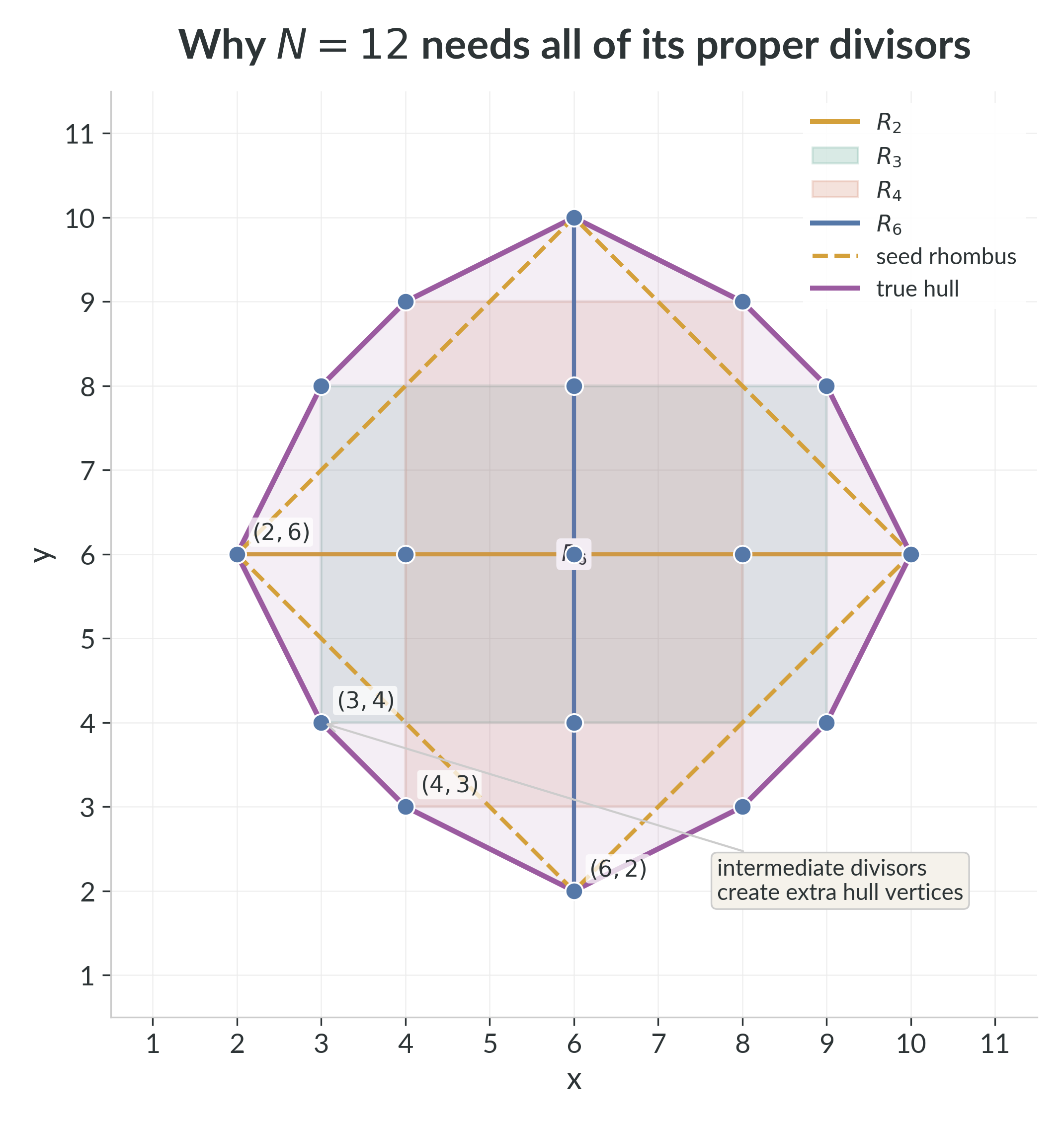
The smallest divisor gives a natural seed shape, but unless the divisor structure is very sparse, intermediate divisors can create additional hull vertices and enlarge the true zero-class hull. The first instructive example is $N=12$. The extreme divisor pair $(2,6)$ and $(6,2)$ suggests a dashed seed rhombus, but the additional divisor points $(3,4)$ and $(4,3)$, together with their reflected partners, push the hull farther out.

@fig:zero-class-n12-anatomy shows exactly where those extra vertices come from. The point of the picture is not only that the hull is larger than the seed rhombus, but that the extra size is created by intermediate divisors rather than by the smallest divisor alone.

Explore interactively

Structural anatomy of the zero class

Theorem (Exact divisor-rectangle description of the zero class). \label{thm:divisor-rectangle-zero-class} Assume that $N$ is composite. Then $$\operatorname{conv}(A_{N,0}) = \operatorname{conv}\!\left( \bigcup_{\substack{d\mid N\\1

Proof. We prove the two containments separately.

First we show $$\operatorname{conv}(A_{N,0}) \subseteq \operatorname{conv}\!\left( \bigcup_{\substack{d\mid N\\1

We claim that $d$ is a proper divisor of $N$. If $d=1$, then $N'=N$, so $N \mid y$, impossible because $1 \leq y \leq N-1$. Also $d

Now $d \mid x$ and $x

For the other containment, fix a proper divisor $d$ of $N$. The four corners $$\left(d,\frac{N}{d}\right), \quad \left(N-d,\frac{N}{d}\right), \quad \left(d,N-\frac{N}{d}\right), \quad \left(N-d,N-\frac{N}{d}\right)$$ all lie in $A_{N,0}$, because each coordinate product is divisible by $N$. Since $R_d$ is the convex hull of these four corners, possibly degenerate to a segment or a point, it follows that $$R_d \subseteq \operatorname{conv}(A_{N,0}).$$ In other words, each divisor rectangle is generated by four genuine zero-class points, so the whole rectangle already lies inside the zero-class hull.

Taking the union over all proper divisors and then taking convex hulls yields $$\operatorname{conv}\!\left( \bigcup_{\substack{d\mid N\\1

\begin{tcolorbox}[enhanced, sharp corners, colback=figurebg, colframe=figureborder, boxrule=0.5pt, left=8pt, right=8pt, top=8pt, bottom=6pt] \small \textbf{Worked check: $N=12$, $(8,9)$.}\quad $d=\gcd(8,12)=4$, $N'=12/4=3$. Because $3 \mid 9$, the divisibility step succeeds. Also $1<4<12$, and $4 \le 8 \le 8$, $3 \le 9 \le 9$. So $(8,9) \in [4,8]\times[3,9] = R_4$. This is the theorem's rectangle-membership argument with concrete numbers filled in. 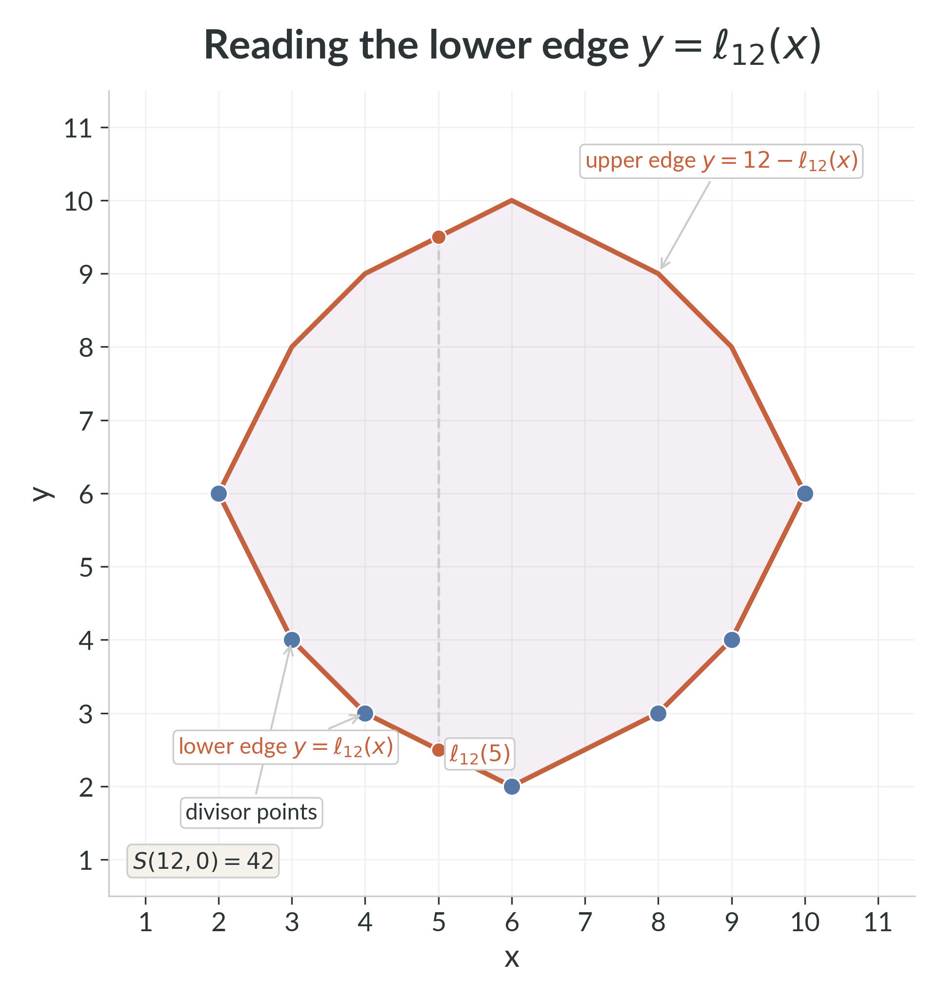\end{tcolorbox}

Remark (Four geometric objects). It is important to distinguish four different sets: $$A_{N,0}, \qquad \bigcup_d R_d, \qquad \operatorname{conv}(A_{N,0}), \qquad \operatorname{conv}\!\left(\bigcup_d R_d\right).$$ The first is a finite lattice set. The second is a filled planar set built from divisor rectangles. The theorem says that the last two convex sets are equal. It does **not** say that the discrete zero class itself equals the rectangle union.

Reading the lower edge of the zero-class hull

The rectangle theorem uses every point of every divisor rectangle. One can describe the same hull more economically by keeping only the lower corners of those rectangles. The lower polygonal chain, or broken line, through those corners controls the whole hull. Here a broken line means a connected chain of straight segments.

We write $\ell_N(x)$ for the height of that lower broken line at horizontal position $x$. In plain language, $\ell_N(x)$ tells us how low the zero-class hull sits above the $x$-axis at the chosen value of $x$.

Definition (Divisor points and the lower edge of the hull). \label{def:zero-class-lower-edge} Assume that $N$ is composite, and let $p$ be the smallest proper divisor of $N$: $$p := \min\{d>1 : d \mid N\}.$$ Define the *divisor point set* $$E_N := \left\{\left(d,\frac{N}{d}\right), \left(N-d,\frac{N}{d}\right) : 1

@fig:zero-class-envelope is the picture to keep in mind. The blue divisor points determine a lower orange broken line; that lower line is $y=\ell_{12}(x)$. The upper orange line is just its reflected partner, and the shaded region between them is the full zero-class hull.

Explore interactively

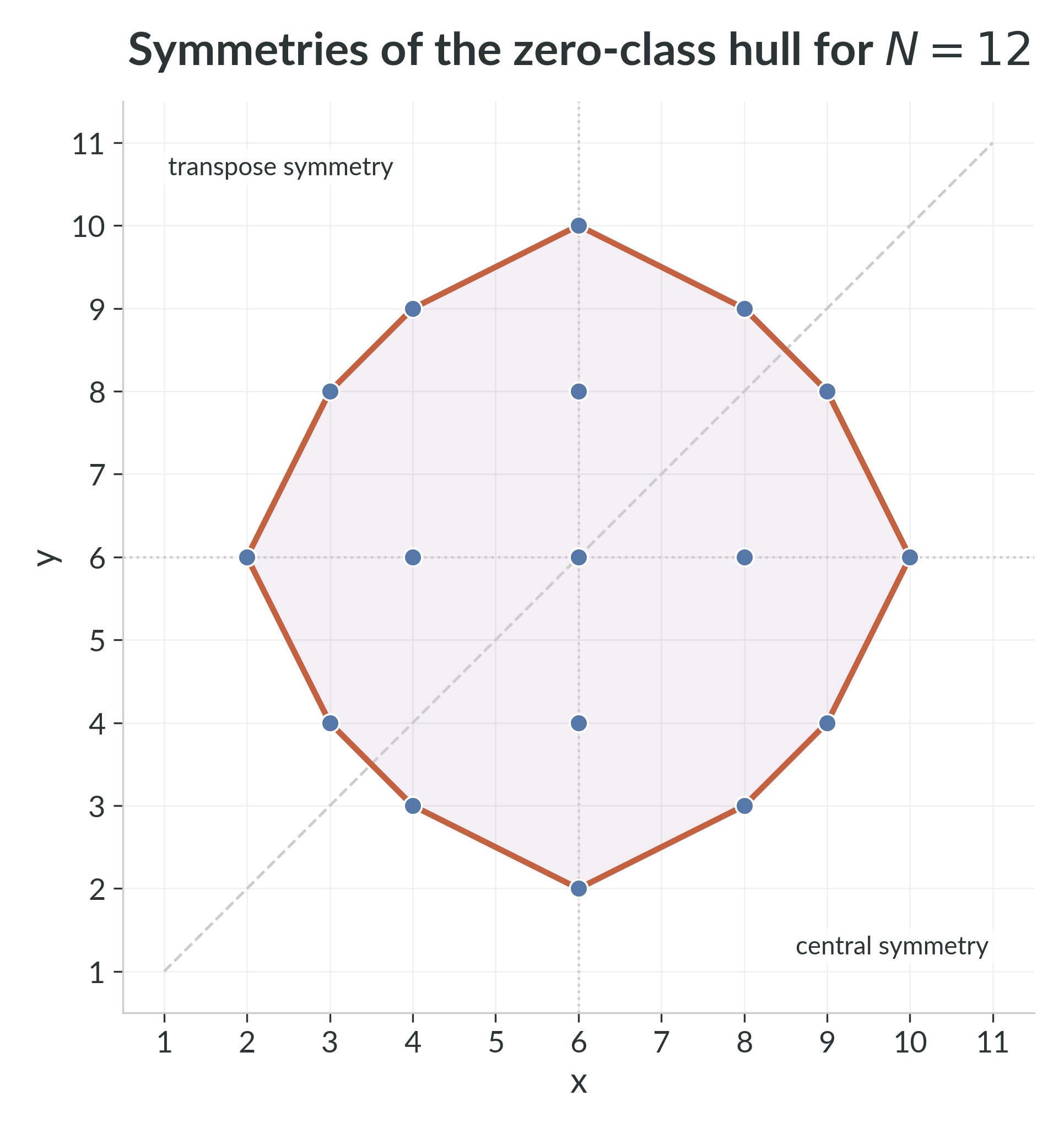
The divisor points already encode the exact lower edge of the zero-class hull. Because $E_N$ is symmetric under $x \mapsto N-x$, the function $\ell_N$ satisfies $$\ell_N(N-x)=\ell_N(x).$$ By the central symmetry from Proposition~\ref{prop:mtmn-symmetries}, the upper boundary of the zero-class hull is therefore the reflected graph $$y = N - \ell_N(x).$$ Transpose symmetry identifies the left and right portions of the hull across the diagonal line $x=y$; central symmetry reflects the lower hull to the upper hull.

Proposition (The hull as the region between two broken lines). \label{prop:zero-class-between-broken-lines} Assume that $N$ is composite. Then $$\operatorname{conv}(A_{N,0}) = \{(x,y) : p \leq x \leq N-p,\ \ell_N(x) \leq y \leq N-\ell_N(x)\}.$$

Proof. Let $$\mathcal{R}_N := \bigcup_{\substack{d\mid N\\1

The key idea is simple: for a fixed $x$-coordinate, the lowest point of the hull is obtained by sliding downward inside the divisor rectangles until one reaches their lower edges. Those lower-edge points are exactly the points that build $\operatorname{conv}(E_N)$.

Take any point $(x,y) \in \operatorname{conv}(\mathcal{R}_N)$. Then $$(x,y)=\sum_{j=1}^m \lambda_j (x_j,y_j)$$ for some convex combination with $(x_j,y_j) \in \mathcal{R}_N$. For each $j$, there exists a proper divisor $d_j$ such that $(x_j,y_j) \in R_{d_j}$. The point $$\left(x_j,\frac{N}{d_j}\right)$$ lies on the lower edge of the same rectangle $R_{d_j}$, so it has the same $x$-coordinate and no larger $y$-coordinate. Moreover, it lies on the horizontal segment joining $$\left(d_j,\frac{N}{d_j}\right) \quad \text{and} \quad \left(N-d_j,\frac{N}{d_j}\right),$$ so it belongs to $\operatorname{conv}(E_N)$.

Therefore the convex combination $$\left(x,\sum_{j=1}^m \lambda_j \frac{N}{d_j}\right)$$ lies in $\operatorname{conv}(E_N)$, has the same $x$-coordinate as $(x,y)$, and has $y$-coordinate at most $y$. This shows that, for each fixed $x$, the smallest possible $y$-coordinate in $\operatorname{conv}(\mathcal{R}_N)$ is exactly the lower boundary of $\operatorname{conv}(E_N)$, namely $\ell_N(x)$.

Because $\operatorname{conv}(A_{N,0})=\operatorname{conv}(\mathcal{R}_N)$ and the zero class is centrally symmetric by Proposition~\ref{prop:mtmn-symmetries}, the upper boundary of $\operatorname{conv}(\mathcal{R}_N)$ is the reflection of the lower boundary under $(x,y) \mapsto (N-x,N-y)$, hence it is given by $y=N-\ell_N(x)$. Since every divisor rectangle satisfies $p \leq x \leq N-p$, the same interval is the full horizontal domain of the hull. The stated description follows. □

@fig:zero-class-symmetry isolates the two Euclidean symmetries used here.

Explore interactively

The same divisor points may also be viewed as samples on the hyperbola $y=N/x$. @fig:zero-class-hyperbola uses that picture only as a guide to intuition: the exact hull comes from the finite divisor data, not from the full continuous curve.

Explore interactively

Corollary (Integral formula for the zero-class area). \label{cor:zero-class-integral-formula} Assume that $N$ is composite. Then $$S(N,0)=\int_p^{N-p}\bigl(N-2\ell_N(x)\bigr)\,dx.$$

Proof. By Proposition~\ref{prop:zero-class-between-broken-lines}, the vertical thickness of the hull at horizontal coordinate $x$ is $$\bigl(N-\ell_N(x)\bigr)-\ell_N(x)=N-2\ell_N(x).$$ Integrating this thickness across the interval $[p,N-p]$ gives the area. □

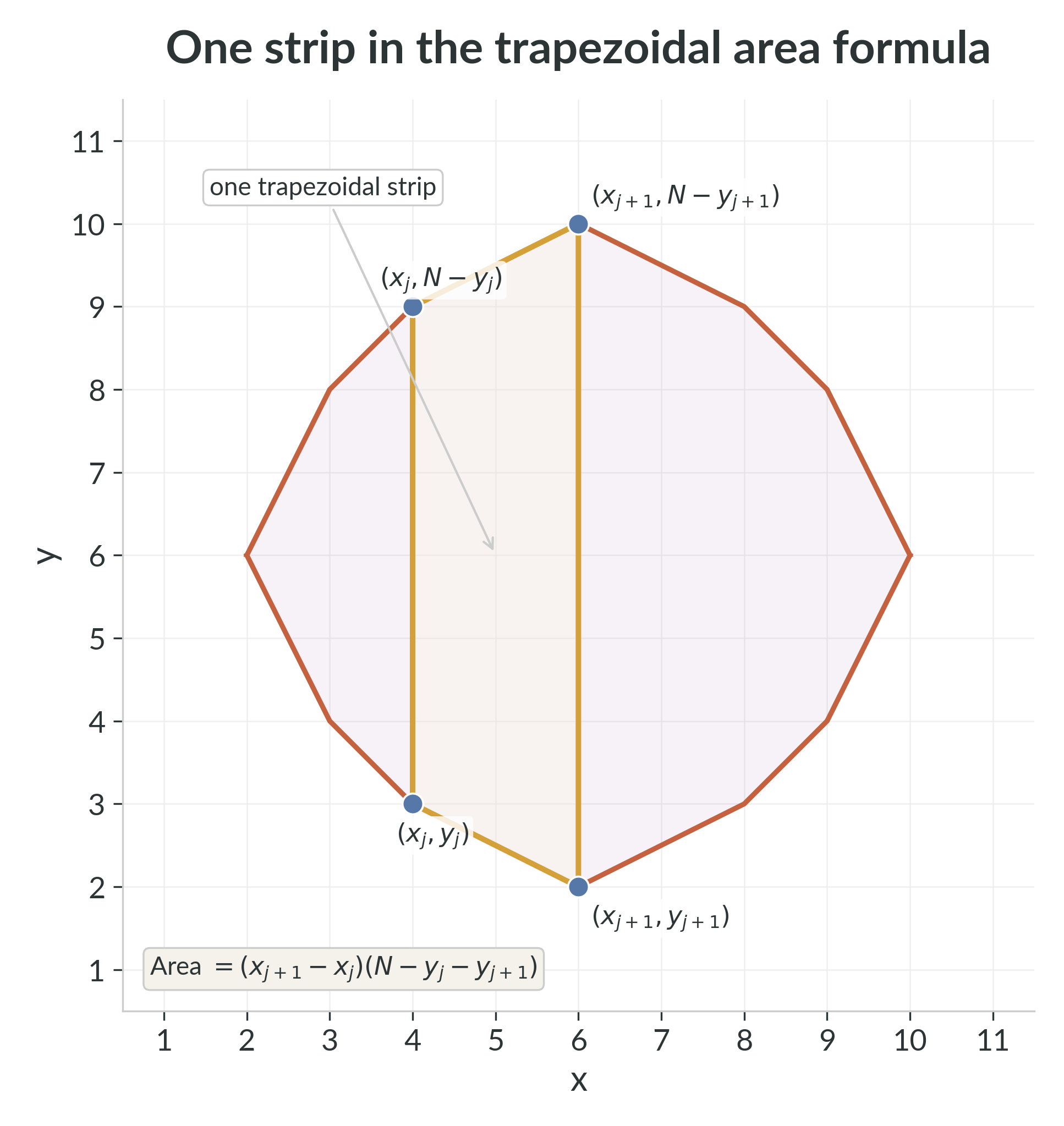
For example, when $N=9$, the only proper divisor is $3$, so the lower edge is the constant line $\ell_9(x)=3$ on the interval $[3,6]$. The integral becomes $$\int_3^6 (9-2\cdot 3)\,dx = \int_3^6 3\,dx = 9,$$ which matches $S(9,0)=9$.

Corollary (Trapezoidal formula for the zero-class area). \label{cor:zero-class-trapezoid-formula} Assume that $N$ is composite, and let the lower-hull vertices of $\operatorname{conv}(E_N)$ be $$v_1=(x_1,y_1),\; v_2=(x_2,y_2),\; \ldots,\; v_r=(x_r,y_r), \qquad x_1=p,\ x_r=N-p,$$ listed from left to right. Then $$S(N,0)=\sum_{j=1}^{r-1}(x_{j+1}-x_j)\bigl(N-y_j-y_{j+1}\bigr).$$

Proof. On each interval $[x_j,x_{j+1}]$, the lower boundary is the line segment joining $(x_j,y_j)$ to $(x_{j+1},y_{j+1})$, and the upper boundary is its reflected partner. The vertical thickness at the two endpoints is $$N-2y_j \qquad \text{and} \qquad N-2y_{j+1}.$$ Hence the area of the strip over that interval is the area of a trapezoid: $$\frac{x_{j+1}-x_j}{2}\bigl((N-2y_j)+(N-2y_{j+1})\bigr) =(x_{j+1}-x_j)\bigl(N-y_j-y_{j+1}\bigr).$$ Summing over all consecutive lower-hull segments gives the formula. □

@fig:zero-class-trapezoid-strip shows one such strip. Each linear piece of the lower hull contributes one reflected trapezoid, and the full area is the sum of those elementary pieces.

Explore interactively

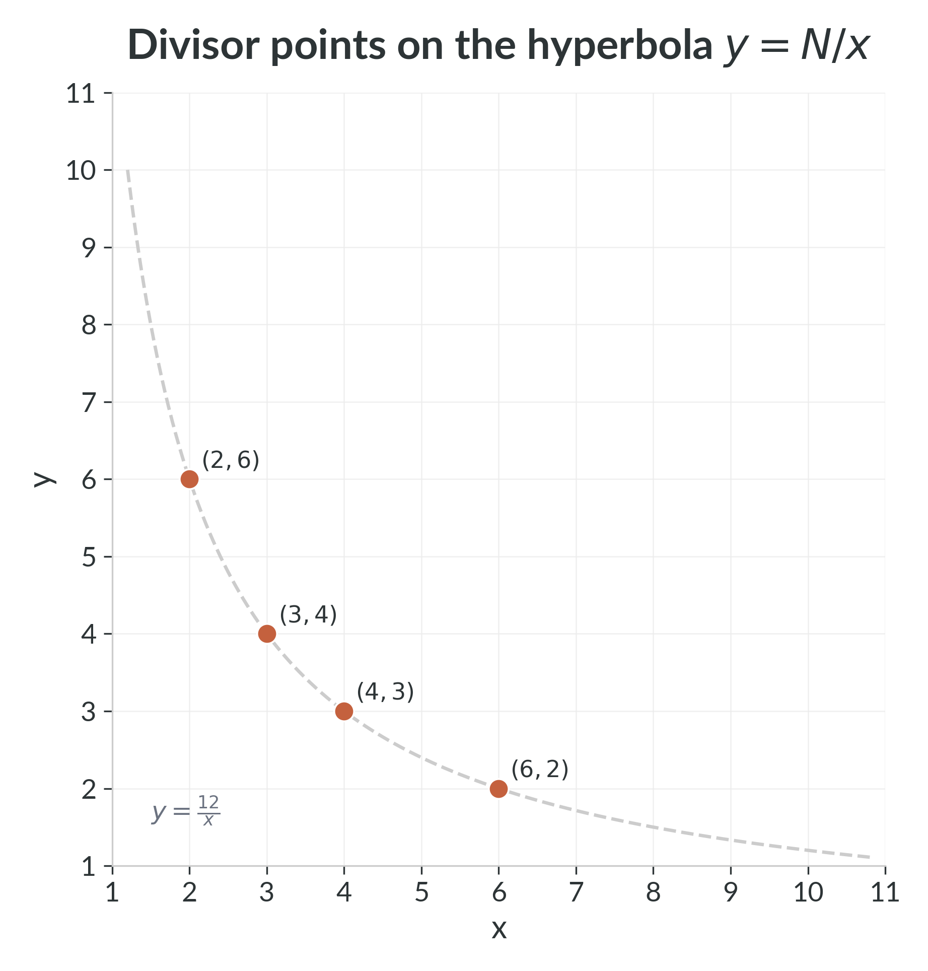
For $N=12$, the lower-hull vertices are $$ (2,6),\ (3,4),\ (4,3),\ (6,2),\ (8,3),\ (9,4),\ (10,6). $$ Therefore Corollary~\ref{cor:zero-class-trapezoid-formula} gives $$ \begin{aligned} S(12,0) &= (3-2)(12-6-4) + (4-3)(12-4-3) + (6-4)(12-3-2) \\ &\quad + (8-6)(12-2-3) + (9-8)(12-3-4) + (10-9)(12-4-6) \\ &= 2 + 5 + 14 + 14 + 5 + 2 \\ &= 42. \end{aligned} $$ This agrees with the exact hull area computed directly from the lattice picture.

The zero class is now understood in two complementary ways. Theorem~\ref{thm:zero-class-degeneracy} gives a clean prime/composite classification of when the hull is degenerate. Theorem~\ref{thm:divisor-rectangle-zero-class} and Corollaries~\ref{cor:zero-class-integral-formula}--\ref{cor:zero-class-trapezoid-formula} explain the full composite geometry: $S(N,0)$ is the area of a completely described divisor-controlled hull.

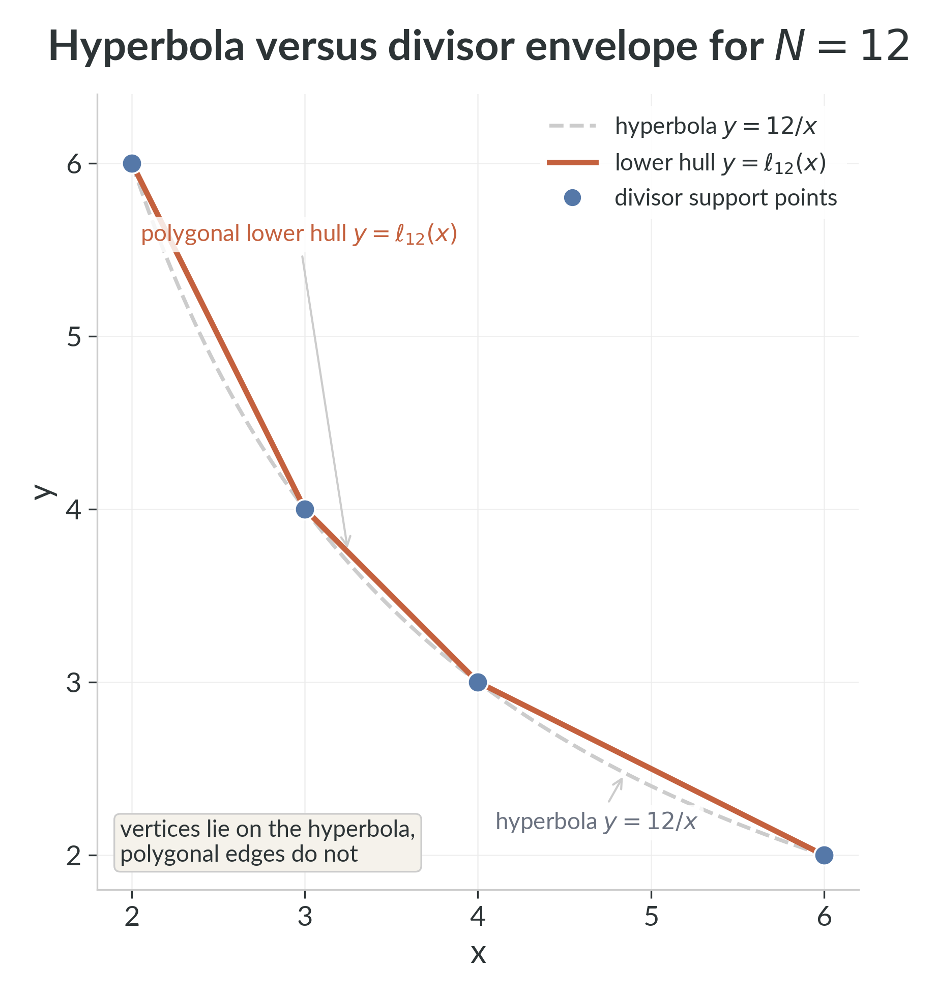
There is one further comparison that now becomes irresistible. The decisive support points $$ \left(d,\frac{N}{d}\right) $$ lie on the continuous hyperbola $$ y=\frac{N}{x}, $$ but the exact hull does not follow that curve. It follows the polygonal divisor envelope. The next question is therefore not whether the hyperbola matters; it is exactly how much area is created when one replaces the smooth curve by the arithmetic polygon.

The hyperbola gap on the informative half

What is true is that the lower-hull support points lie on the hyperbola $y=N/x$. What is not true is that every point of the lower hull lies on that hyperbola. The hull is the polygonal lower convex envelope of the sampled divisor points, so its edges are straight secants rather than curved arcs. @fig:zero-class-hyperbola-vs-hull-n12 shows this directly for $N=12$: the vertices lie on the curve, but the orange segments do not.

Explore interactively

Proposition (The divisor envelope lies above the hyperbola). \label{prop:zero-class-envelope-above-hyperbola} Assume that $N$ is composite. Then on the informative left half, $$ \ell_N(x) \geq \frac{N}{x} \qquad \text{for } p \leq x \leq \frac{N}{2}. $$

Proof. The function $$ f(x)=\frac{N}{x} $$ has second derivative $$ f''(x)=\frac{2N}{x^3}>0 $$ for $x>0$, so its graph is convex. Therefore, whenever one takes two divisor points $$ \left(d_j,\frac{N}{d_j}\right), \qquad \left(d_{j+1},\frac{N}{d_{j+1}}\right) $$ that appear consecutively on the left lower hull, the secant line joining them lies above the graph of $y=N/x$ on the whole interval $[d_j,d_{j+1}]$.

Those secant lines are exactly the linear pieces of $\ell_N$ until the symmetry point is reached. If $N$ is odd, there is one final interval from the last left-side divisor vertex to $x=N/2$ on which the lower hull is horizontal. Since $x \mapsto N/x$ is decreasing, the hyperbola also lies below that horizontal segment. 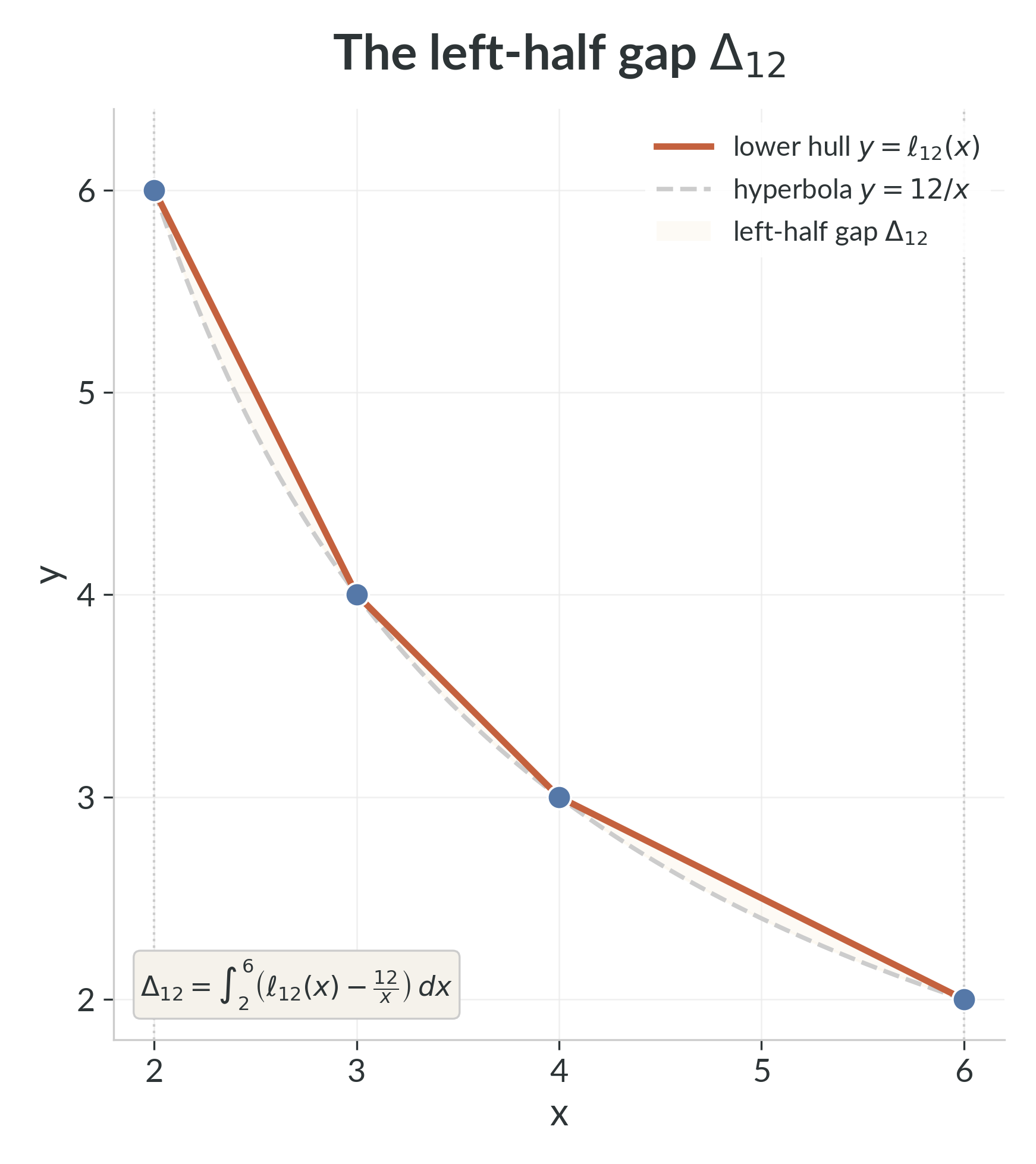Hence every piece of the left lower hull lies on or above the hyperbola, so $$ \ell_N(x) \geq \frac{N}{x} $$ throughout $[p,N/2]$. □

This order of subtraction is therefore the correct one: the hyperbola is the lower continuous model, while the divisor envelope is the higher polygonal arithmetic model.

Definition (The left-half hyperbola gap). \label{def:zero-class-hyperbola-gap} Assume that $N$ is composite. Define $$ \Delta_N := \int_p^{N/2}\left(\ell_N(x)-\frac{N}{x}\right)\,dx. $$

By Proposition~\ref{prop:zero-class-envelope-above-hyperbola}, the integrand is everywhere nonnegative, so $$ \Delta_N \geq 0. $$ Geometrically, $\Delta_N$ is the area between the polygonal lower hull and the continuous hyperbola on the informative half of the picture. The shaded region in @fig:zero-class-delta-left-half-n12 is exactly that area for $N=12$.

Explore interactively

Decomposing the gap segment by segment

Because $\ell_N$ is piecewise linear, the total gap breaks into the sum of the smaller regions trapped between each hull segment and the hyperbola.

Let $$ p=x_1

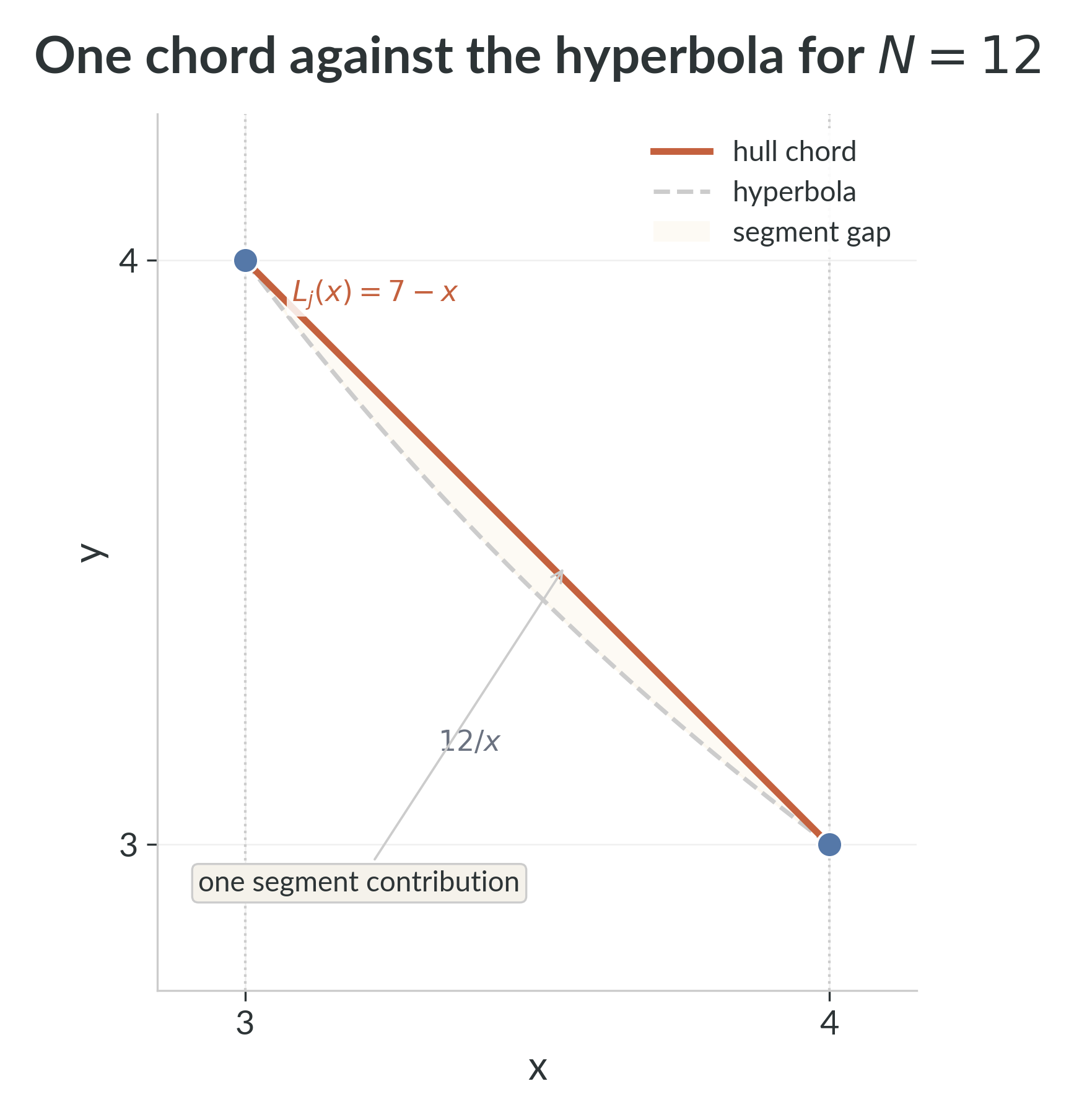
Proposition (Piecewise decomposition of the hyperbola gap). \label{prop:zero-class-gap-piecewise} With the notation above, $$ \Delta_N = \sum_{j=1}^{t-1} \int_{x_j}^{x_{j+1}} \left(L_j(x)-\frac{N}{x}\right)\,dx. $$

Proof. On each interval $[x_j,x_{j+1}]$, the lower hull agrees with the linear function $L_j$. Splitting the integral for $\Delta_N$ across those consecutive intervals gives the stated sum. □

When both endpoints of one interval are genuine divisor vertices, the line has a particularly simple form. Suppose $$ \left(d_j,\frac{N}{d_j}\right), \qquad \left(d_{j+1},\frac{N}{d_{j+1}}\right) $$ are consecutive left-side divisor vertices joined by one segment of the lower hull. Then on $[d_j,d_{j+1}]$, $$ L_j(x) = \frac{N}{d_j} + \frac{\frac{N}{d_{j+1}}-\frac{N}{d_j}}{d_{j+1}-d_j}(x-d_j). $$ This is the local picture isolated in @fig:zero-class-segment-gap-n12.

Explore interactively

Proposition (A closed formula for one divisor-to-divisor segment). \label{prop:zero-class-gap-segment-formula} In the divisor-to-divisor situation above, $$ \int_{d_j}^{d_{j+1}} L_j(x)\,dx = \frac{d_{j+1}-d_j}{2}\left(\frac{N}{d_j}+\frac{N}{d_{j+1}}\right), $$ $$ \int_{d_j}^{d_{j+1}} \frac{N}{x}\,dx = N\ln\left(\frac{d_{j+1}}{d_j}\right), $$ and therefore $$ \int_{d_j}^{d_{j+1}} \left(L_j(x)-\frac{N}{x}\right)\,dx = \frac{d_{j+1}-d_j}{2}\left(\frac{N}{d_j}+\frac{N}{d_{j+1}}\right) -N\ln\left(\frac{d_{j+1}}{d_j}\right). $$

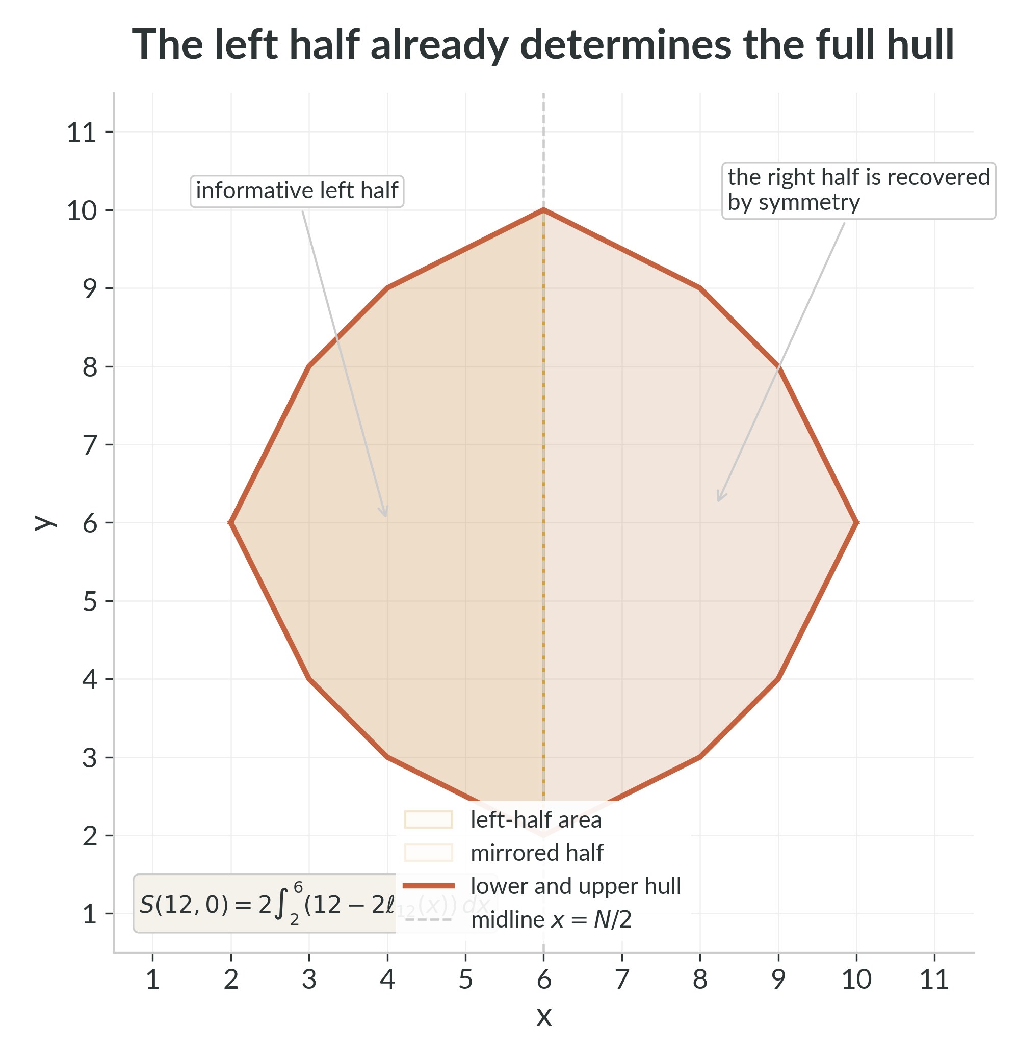
Proof. The integral of a line over an interval is the area of the corresponding trapezoid, so $$ \int_{d_j}^{d_{j+1}} L_j(x)\,dx = \frac{d_{j+1}-d_j}{2}\left(\frac{N}{d_j}+\frac{N}{d_{j+1}}\right). $$ Also $$ \int_{d_j}^{d_{j+1}} \frac{N}{x}\,dx = N\bigl[\ln x\bigr]_{d_j}^{d_{j+1}} = N\ln\left(\frac{d_{j+1}}{d_j}\right). $$ Subtracting gives the segment formula. □

Remark (A ratio form). On a divisor-to-divisor interval it is natural to write $$ r_j:=\frac{d_{j+1}}{d_j}. $$ Then $$ \frac{d_{j+1}-d_j}{2}\left(\frac{N}{d_j}+\frac{N}{d_{j+1}}\right) = N\cdot \frac{r_j-1}{2}\left(1+\frac{1}{r_j}\right), $$ so the same segment contribution becomes $$ N\,F(r_j), \qquad F(r):=\frac{r-1}{2}\left(1+\frac{1}{r}\right)-\ln r. $$ Thus each divisor-to-divisor gap contributes an amount determined only by the ratio of successive divisor abscissas, scaled by $N$.

Remark (If the midpoint is not itself a divisor point). For odd $N$, the last left-half interval runs from the final divisor vertex to $x=N/2$ and is horizontal rather than divisor-to-divisor. Proposition~\ref{prop:zero-class-gap-piecewise} still applies exactly, and the same trapezoid-minus-log calculation still evaluates that last piece. The ratio formula above is simply the cleanest form for the intervals whose endpoints are both sampled divisor points.

Exact relation with the zero-class area

The point of $\Delta_N$ is that it measures the exact difference between the true hull area and the area one would obtain by pretending that the lower boundary were the continuous hyperbola itself. By symmetry, the left half already determines the full area, as @fig:zero-class-gap-symmetry-n12 makes visible.

Explore interactively

Theorem (Exact hyperbolic decomposition of the zero-class area). \label{thm:zero-class-hyperbola-gap-identity} Assume that $N$ is composite. Then $$ S(N,0)=N(N-2p)-4N\ln\left(\frac{N}{2p}\right)-4\Delta_N. $$ Equivalently, $$ \Delta_N = \frac{1}{4}\left[ N(N-2p)-4N\ln\left(\frac{N}{2p}\right)-S(N,0) \right]. $$

Proof. Corollary~\ref{cor:zero-class-integral-formula} gives $$ S(N,0)=\int_p^{N-p}\bigl(N-2\ell_N(x)\bigr)\,dx. $$ Because $\ell_N(N-x)=\ell_N(x)$, the integrand is symmetric about $x=N/2$, so $$ S(N,0)=2\int_p^{N/2}\bigl(N-2\ell_N(x)\bigr)\,dx. $$ Now write $$ \ell_N(x)=\frac{N}{x}+\left(\ell_N(x)-\frac{N}{x}\right). $$ Then $$ N-2\ell_N(x) = \left(N-\frac{2N}{x}\right)-2\left(\ell_N(x)-\frac{N}{x}\right). $$ Substituting into the integral gives $$ S(N,0) = 2\int_p^{N/2}\left(N-\frac{2N}{x}\right)\,dx -4\int_p^{N/2}\left(\ell_N(x)-\frac{N}{x}\right)\,dx. $$ The second integral is exactly $\Delta_N$. The first is $$ 2\left[ Nx-2N\ln x \right]_{p}^{N/2} = N(N-2p)-4N\ln\left(\frac{N}{2p}\right). 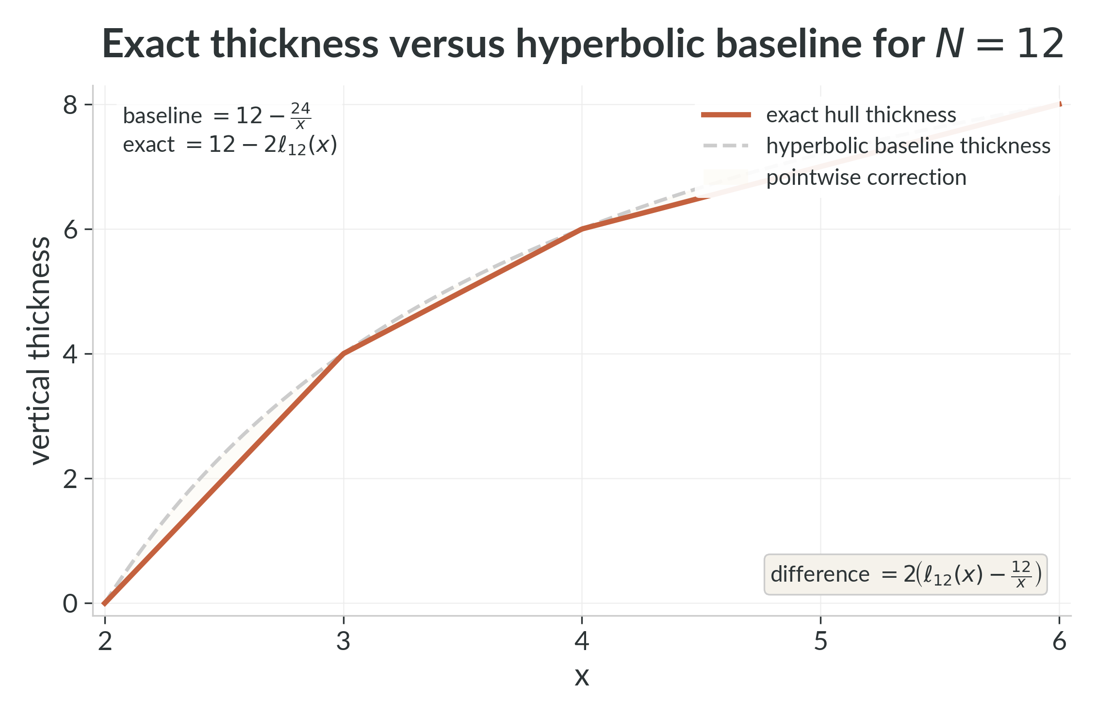$$ Combining the two terms proves the stated identity. □

Remark (Baseline and correction). The term $$ N(N-2p)-4N\ln\left(\frac{N}{2p}\right) $$ is the area obtained by replacing the exact thickness $$ N-2\ell_N(x) $$ with the smoother hyperbolic thickness $$ N-\frac{2N}{x} $$ on the informative half and then reflecting by symmetry. The exact area is that hyperbolic baseline minus the correction $4\Delta_N$. This is not an approximation claim. It is an exact geometric decomposition of the zero-class area into a continuous term and an arithmetic polygonal correction.

This comparison sits beside the same classical hyperbolic backdrop as the Dirichlet divisor problem, where one studies lattice-point data attached to the region under $xy=N$, equivalently under the graph $y=N/x$ [@ivickratzelkuehleitnernowak2004]. The object measured here is different, however. The term $\Delta_N$ is not a summatory divisor error term, but the exact area between the smooth hyperbola and the polygonal divisor envelope that governs the zero-class hull for one fixed modulus.

The pointwise version of that correction is drawn in @fig:zero-class-thickness-comparison-n12: the exact thickness curve sits above the hyperbolic baseline by twice the local gap $\ell_N(x)-N/x$.

Explore interactively

Worked example: $N=12$

For $N=12$, the informative left-half lower-hull vertices are $$ (2,6),\ (3,4),\ (4,3),\ (6,2). $$ Hence $$ \ell_{12}(x)=10-2x \qquad \text{for } 2 \leq x \leq 3, $$ $$ \ell_{12}(x)=7-x \qquad \text{for } 3 \leq x \leq 4, $$ and $$ \ell_{12}(x)=5-\frac{x}{2} \qquad \text{for } 4 \leq x \leq 6. $$ Therefore $$ \Delta_{12} = \int_2^3\left(10-2x-\frac{12}{x}\right)\,dx + \int_3^4\left(7-x-\frac{12}{x}\right)\,dx + \int_4^6\left(5-\frac{x}{2}-\frac{12}{x}\right)\,dx. $$

Evaluating each piece gives $$ \int_2^3\left(10-2x-\frac{12}{x}\right)\,dx = 5-12\ln\left(\frac{3}{2}\right), $$ $$ \int_3^4\left(7-x-\frac{12}{x}\right)\,dx = \frac{7}{2}-12\ln\left(\frac{4}{3}\right), $$ and $$ \int_4^6\left(5-\frac{x}{2}-\frac{12}{x}\right)\,dx = 5-12\ln\left(\frac{3}{2}\right). $$ Summing yields $$ \Delta_{12} = \frac{27}{2} -12\left(2\ln\left(\frac{3}{2}\right)+\ln\left(\frac{4}{3}\right)\right) = \frac{27}{2}-12\ln 3. $$

The hyperbolic baseline term is $$ H_{12}:=12(12-4)-48\ln 3=96-48\ln 3. $$ Theorem~\ref{thm:zero-class-hyperbola-gap-identity} therefore gives $$ \begin{aligned} S(12,0) &= H_{12}-4\Delta_{12} \\ &= (96-48\ln 3)-4\left(\frac{27}{2}-12\ln 3\right) \\ &= 42. \end{aligned} $$ This matches the earlier trapezoidal calculation exactly. So the two pictures agree perfectly: the full hull area is $42$, and the quantity $$ \Delta_{12}=\frac{27}{2}-12\ln 3 $$ is precisely the arithmetic correction that converts the smooth hyperbolic baseline into that exact polygonal area.

The zero class is now understood in three compatible ways: as a divisor-rectangle hull, as a region between the broken lines $y=\ell_N(x)$ and $y=N-\ell_N(x)$, and as a hyperbolic baseline corrected by the nonnegative gap term $\Delta_N$. The next chapter changes the language rather than the object: it keeps the same finite residue classes, but recasts their areas through support functions and exact integral formulas.