Background and notation

Conventions on integers and residues

Throughout the book, the modulus $N$ and the coordinates $x,y$ are positive integers. Residues are represented by the set $$\{0,1,\ldots,N-1\},$$ so the residue label $a$ may be zero even though the lattice coordinates are positive.

Later, when we compare modular classes with ordinary hyperbolas, we will do so inside the same positive window by tracking the exact products $a+kN$ that occur there.

Modular arithmetic

When we write $$xy \equiv a \pmod{N},$$ we mean that $N$ divides $xy - a$. Equivalently, $xy$ and $a$ leave the same remainder upon division by $N$. The set of residues modulo $N$ is $$\mathbb{Z}/N\mathbb{Z} = \{0, 1, \ldots, N-1\}$$ with arithmetic performed modulo $N$. This congruence language was organized systematically by Gauss in Disquisitiones Arithmeticae [@gauss1801].

We will say that a number $u$ is coprime to $N$ if $\gcd(u,N)=1$, meaning that $u$ and $N$ share no common factor greater than $1$. Equivalently, $u$ is invertible modulo $N$: there exists some residue $v$ with $uv \equiv 1 \pmod{N}$.

Lattice points and convex hulls

A lattice point in the plane is simply a point of $\mathbb{Z}^2$. The finite square $$\{1, \ldots, N-1\}^2$$ may be viewed as a Euclidean lattice window. For any finite set $E \subset \mathbb{R}^2$, the convex hull $\operatorname{conv}(E)$ is the smallest convex set containing $E$. Geometrically, if one places nails at the points of $E$ and stretches a rubber band around them, the rubber band traces the boundary of $\operatorname{conv}(E)$.

Area

For a polygon with ordered vertices $(x_1, y_1), \ldots, (x_m, y_m)$ listed cyclically (with the convention that $(x_{m+1}, y_{m+1}) = (x_1, y_1)$), the shoelace formula states $$\operatorname{Area}(P) = \frac{1}{2} \left| \sum_{j=1}^{m} (x_j y_{j+1} - x_{j+1} y_j) \right|.$$

\begin{minipage}[t]{0.56\linewidth} \vspace{0pt} This will be our main exact tool once the hull vertices are known. For an MTMN example, the residue class $$A_{5,1}=\{(1,1),(2,3),(3,2),(4,4)\}$$ has convex-hull vertices in cyclic order. The companion picture marks those four points and the cyclic hull order used in the computation: $$ (1,1), \ (3,2), \ (4,4), \ (2,3). $$ Therefore \begin{align} &\operatorname{Area}(\operatorname{conv}(A_{5,1})) \ &= \tfrac{1}{2}\bigl|(1{\cdot}2 + 3{\cdot}4 + 4{\cdot}3 + 2{\cdot}1) - (1{\cdot}3 + 2{\cdot}4 + 4{\cdot}2 + 3{\cdot}1)\bigr| \ &= \tfrac{1}{2}|28-22| = 3. \end{align} So $S(5,1)=3$. \end{minipage}\hfill \begin{minipage}[t]{0.38\linewidth} \vspace{0pt} \begin{MTMNFigureCard} \includegraphics[width=\linewidth]{figures/a51_shoelace_example.png} \captionof{figure}{The residue class $A_{5,1}$ and the convex hull used in the shoelace computation.} \end{MTMNFigureCard} \end{minipage}

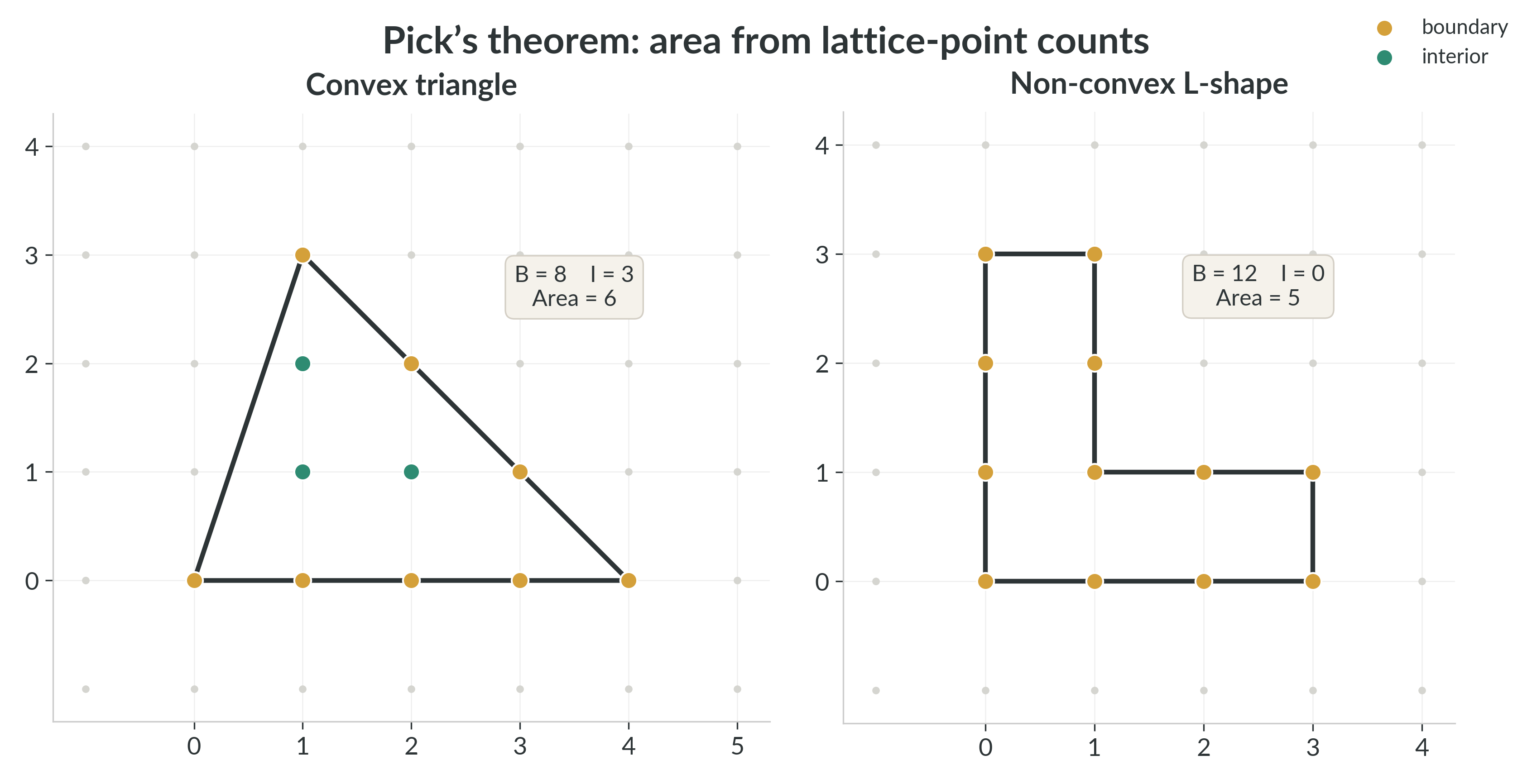
A second standard fact, useful when the polygon is already explicit as a lattice polygon, is Pick's theorem [@pick1899]: $$\operatorname{Area}(P) = I(P) + \frac{B(P)}{2} - 1,$$ where $I(P)$ is the number of interior lattice points and $B(P)$ is the number of lattice points on the boundary of $P$. Pick's theorem computes the area of any simple lattice polygon -- convex or not -- purely by counting lattice points, with no need for coordinate decomposition or trigonometry. We will use it mainly as a structural tool: it relates area to lattice counts, but it does not by itself tell us which lattice points form the hull.

@fig:picks-examples shows two examples. On the left, a triangle with vertices $(0,0)$, $(4,0)$, $(1,3)$ has $B = 8$ boundary points and $I = 3$ interior points, giving $\operatorname{Area} = 3 + 8/2 - 1 = 6$. On the right, an L-shaped non-convex polygon has $B = 12$ and $I = 0$, giving $\operatorname{Area} = 0 + 12/2 - 1 = 5$. The second example illustrates that Pick's theorem applies even when the shape is not convex.

Historically, the formula goes back to Pick's 1899 paper [@pick1899].

Indicator notation and exponential filters

For a statement $C$, the indicator function $\mathbf{1}_C$ equals $1$ when $C$ is true and $0$ otherwise. Thus $$\mathbf{1}_{xy \equiv a \pmod{N}} = \begin{cases} 1, & xy \equiv a \pmod{N}, \\ 0, & \text{otherwise}. \end{cases}$$

A standard Fourier identity on the finite cyclic group $\mathbb{Z}/N\mathbb{Z}$ is $$\mathbf{1}_{xy \equiv a \pmod{N}} = \frac{1}{N} \sum_{r=0}^{N-1} \exp\!\left(\frac{2\pi i r(xy - a)}{N}\right).$$ This identity is exact: if $xy - a \equiv 0 \pmod{N}$, every exponential equals $1$ and the average is $1$; otherwise the $N$ roots of unity cancel to $0$.

For example, when $N = 4$ the four 4th roots of unity are $1,\; i,\; -1,\; -i$. Their sum is $$1 + i + (-1) + (-i) = 0,$$ because opposite terms cancel in pairs. The same cancellation occurs for any $N$: the $N$-th roots of unity are equally spaced around the unit circle, and unless every term equals $1$ (which happens exactly when $xy \equiv a$), their symmetric arrangement forces the sum to vanish.